You can define a symbol to be a random variable and then query that random variable for information, or sample that random variable. There are many such continuous distributions programmed into Maple, but we will look at only a few that are relevant to engineering.
[> with( Statistics ):
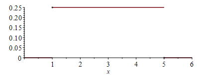
This is a continuous distribution where there is an equal likelihood of a value appearing between two numbers $a < b$.
[> X1 := RandomVariable( 'Uniform( a, b )' ):
[> Mean( X1 );
$\frac{a}{2} + \frac{b}{2}$
[> StandardDeviation( X1 );
$\frac{\sqrt{3} \sqrt{ (b - a)^2 } }{6}$
We can ask Maple for the probability density function and the cummulative distribution functions:
[> PDF( X1 );
$\left \{ \begin{matrix} 0 & x < a \\ \frac{1}{b - a} & x < b \\ 0 & \textit{otherwise} \end{matrix} \right .$
[> CDF( X1 );
$\left \{ \begin{matrix} 0 & x < a \\ \frac{x - a}{b - a} & x < b \\ 1 & \textit{otherwise} \end{matrix} \right .$
[> X1f := RandomVariable( 'Uniform( 1, 5 )' ):
[> Mean( X1f );
$3$
[> StandardDeviation( X1f );
$\frac{2\sqrt{3}}{3}$
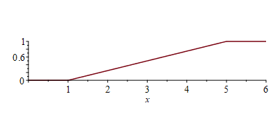
The probability density function is discontinuous, so we should use the 'discont' = true option:
[> plot( PDF( X1f, x ), x = 0..6, 'discont' = true );
[> plot( CDF( X1f, x ), x = 0..6, 'discont' = true );
[> f1 := Sample( X1f ):
[> f1( 10 );
$[3.6203920158953626, 1.6504469407785223, 1.4759907262335066, 2.993456207928572,$ $4.838975834064325, 2.361542906664533, 3.3410710039191094, 1.895247757964548,$ $4.005068237222611, 2.0203804618370764]$
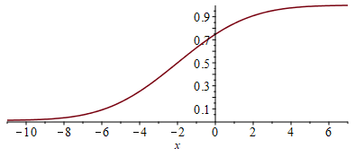
This is a continuous distribution equivalent to the usual bell curve with a given mean and standard deviation:
[> X2 := RandomVariable( 'Normal( mu, sigma )' ):
[> Mean( X2 );
$\mu$
[> StandardDeviation( X2 );
$\sigma$
We can ask Maple for the probability density function and the cummulative distribution functions:
[> PDF( X2 );
$\frac{\sqrt{2}e^{-\frac{(x - \mu)^2}{2\sigma^2}}}{2\sqrt{\pi} \sigma}$
[> CDF( X2 );
$\frac{1}{2} + \frac{\textrm{erf} \left({\frac { \left( x-\mu \right) \sqrt {2} }{2 \sigma}}\right)}{2} $
[> X2f := RandomVariable( 'Normal( -2, 3 )' ):
[> Mean( X2f );
$-2$
[> StandardDeviation( X2f );
$3$
[> plot( PDF( X2f, x ), x = -11..7 );

[> plot( CDF( X2f, x ), x = -11..7 );
[> f2 := Sample( X2f ):
[> f2( 10 );
$[1.2017008485503808, 2.2060565876883977, -4.162598640192476, -6.1174844206463295,$ $-0.35191374398380093, -2.0501804170515747, 1.8729911446438114, -1.2366724530815374,$ $-3.1180144880897274, -1.739101963430866]$
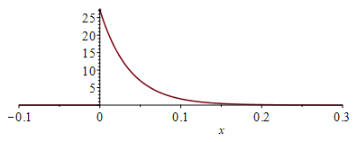
This is a continuous distribution that describes the time between independent events when the average time between events is $b$. So for example, if a call center receives 27.2 calls per hour, then the average time between calls must be $\frac{1}{27.2} \approx 0.03676470588$ hours or 2 minutes and 12 seconds; however, the time between any two events is not going to be exactly 2 minutes and 12 seconds. The exponential distribution describes the time intervals between such events.
[> X3 := RandomVariable( 'Exponential( delta )' ):
[> Mean( X3 );
$\delta$
[> StandardDeviation( X3 );
$\delta$
We can ask Maple for the probability density function and the cummulative distribution functions:
[> PDF( X3 );
$\left \{ \begin{matrix} 0 & x < 0 \\ \frac{e^{-\frac{x}{\delta}}}{\delta} \end{matrix} \right.$
[> CDF( X3 );
$\left \{ \begin{matrix} 0 & x < 0 \\ 1 - e^{-\frac{x}{\delta}} \end{matrix} \right.$
[> X3f := RandomVariable( 'Exponential( 1/27.2 )' ):
[> Mean( X3f );
$0.03676470588$
[> StandardDeviation( X3f );
$0.03676470587$
[> plot( PDF( X3f, x ), x = -0.1..0.3 );
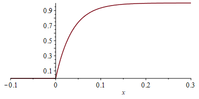
[> plot( CDF( X3f, x ), x = -0.1..0.3 );
[> f3 := Sample( X3f ):
[> f3( 10 );
$[0.008031484705298806, 0.030336664409757984, 0.013972451141163746,$ $0.054243172757515196, 0.018605132125918897, 0.03721196813390189,$ $0.04405742115148007, 0.0296437772133251, 0.032649770843399296,$ $0.009336955869392616]$