You can define a symbol to be a random variable and then query that random variable for information, or sample that random variable. There are many such distributions programmed into Maple, but we will look at only a few that are relevant to engineering.
[> with( Statistics ):
This is the flip of a weighted coin, with $1$ coming up with a probability of $p$ and $0$ coming up with a probability of $1 - p$. It is therefore a discrete distribution.
[> X1 := RandomVariable( 'Bernoulli( p )' ):
[> Mean( X1 );
$p$
[> StandardDeviation( X1 );
$\sqrt{ p(1 - p) }$
[> X1f := RandomVariable( 'Bernoulli( 0.8 )' ):
[> Mean( X1f );
$0.8$
[> StandardDeviation( X1f );
$0.4$
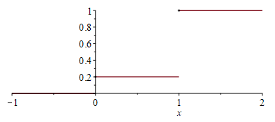
The cummulative distribution function for a discrete distribution is discontinuous, so we should pass the option 'discont' = true:
[> plot( CDF( X1f, x ), x = -1..2, 'discont' = true );
The Sample( n ) function returns $n$ samples from the distribution stored by default in a vector:
[> f1 := Sample( X1f ):
[> f1( 10 );
$[1.0, 0., 0., 1.0, 1.0, 0., 1.0, 1.0, 1.0, 1.0]$
This is the result of $n$ flips of a weighted coin, with $1$ coming up with a probability of $p$ and $0$ coming up with a probability of $1 - p$.
[> X2 := RandomVariable( 'Binomial( 5, p )' ):
[> Mean( X2 );
$5p$
[> StandardDeviation( X2 );
$\sqrt{5} \sqrt{ p(1 - p) }$
[> X2f := RandomVariable( 'Binomial( 5, 0.8 )' ):
[> Mean( X2f );
$4.0$
[> StandardDeviation( X2f );
$0.8944271910$
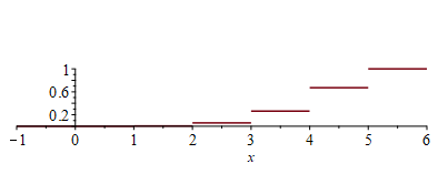
The cummulative distribution function for a discrete distribution is discontinuous, so we should pass the option 'discont' = true:
[> plot( CDF( X2f, x ), x = 0..6, 'discont' = true );
[> f2 := Sample( X2f ):
[> f2( 10 );
$[5. 5. 5. 4. 2. 3. 5. 5. 4. 5.]$
Suppose that a business gets $\lambda = 27.2$ phone calls per hour beteween 1 pm and 5 pm. These phone calls are likely independent, so in some one-hour periods, the business may get 24 calls, and in others, it may get 31 calls. It's less likely, however, for the business to get only 5 calls in any one-hour period, and it's also unlikely that there would be 50 calls per hour. The Poisson distribution with $\lambda$ describes the likelihood of there being $n$ calls in that hours for this specific $\lambda$.
[> X3 := RandomVariable( 'Poisson( lambda )' ):
[> Mean( X3 );
$\lambda$
[> StandardDeviation( X3 );
$\sqrt{ \lambda }$
We can ask Maple for the cummulative distribution functions:
[> CDF( X3 );
$\sum _{i=0}^{\max \left( -1,\left\lfloor x\right\rfloor \right) }{ \frac {{\lambda}^{i}{{\rm e}^{-\lambda}}}{i!}} $
[> X3f := RandomVariable( 'Poisson( 27.2 )' ):
[> Mean( X3f );
$27.2$
[> StandardDeviation( X3f );
$5.215361924$
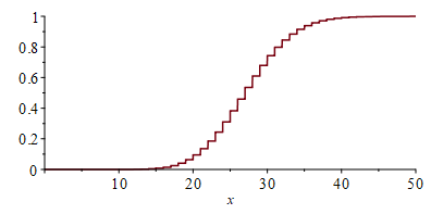
The probability density function is discontinuous, but Maple is not able to find the discontinuities (at this point), so we still see a stairstep function:
[> plot( CDF( X3f, x ), x = 0..50, 'discont' = true );
[> f3 := Sample( X3f ):
[> f3( 10 );
$[26.0, 26.0, 27.0, 25.0, 23.0, 19.0, 26.0, 38.0, 31.0, 23.0]$