
The graph theory package in Maple (GraphTheory) at first looks ominous and daunting with 225 functions and three sub-packages. We'll look at some of the more common functions and features here.
There are two functions in the GraphTheory package used to create graphs: Graph(...) is used to create undirected graphs, and Digraph(...) is used to create directed graphs. With this package, is is probably best to include the package while using it.
The vertices are passed as the first argument, and each vertex may be identified by either a symbol or an indexed name, an integer, or a string. In general, of course, it is likely best if you choose one and only one format per graph. The identifiers of the vertices are passed as a list to either the Graph([...], ...) or Digraph([...], ...) function. As a shorthand, a positive integer n is equivalent to the first argument [1, 2, 3, ..., n].
Recommendation: If you intend to draw the graph, use one- or two-character strings but place all these into an array first so that you can easily switch between integers and the strings:
[> # The list ["A", ..., "Z"]:
[> vA := [seq( StringTools['Char']( k ), k = 65..90 )]:
[> #  - Use va := [seq( ..., k = 97..122 )]: for ["a", ..., "z"]
The following creates all possible pairs ["AA", "AB", ..., "AZ", "BA", ..., "YZ", "ZA", ..., "ZZ"] (676):
[> vAA := [seq( seq(
    cat( StringTools['Char']( k1 ), StringTools['Char']( k2 ) ),
    k2 = 65..90
), k1 = 65..90 )]:
The following creates all possible pairs ["A0", "A1", ..., "A9", "B0", ..., "Y9", "Z0", ..., "Z9"] (260):
[> vA0 := [seq( seq(
    cat( StringTools['Char']( k1 ), k2 ), k2 = 0..9
), k1 = 65..90 )]:
We will look at working with
You can now use these lists to create an undirected graph with a specific number of nodes; for example, this one has ten vertices labelled "J" through "T":
[> with( GraphTheory ):
[> UG := Graph( vA[1..10] ):
In an undirected graph, Maple refers to connections between vertices to be edges, while connections in a directed graph are arcs.
You can either add edges using either a second argument of a set of sets of pairs representing edges, or you can subsequently add edges to an undirected graph by calling the AddEdge(...) function. The following two are equivalent: either creating the graph with the edges, or adding the edges later:
[> UG := Graph( vA[1..10], {{"A", "B"}, {"D", "G"}} ):
[> UG := Graph( vA[1..10] ):
[> AddEdge( UG, {{"A", "B"}, {"D", "G"}} ):
[> Edges( UG );
${{"A", "B"}, {"D", "G"}}$
If you are only adding one edge, you can just pass a single set with the two vertices. If the set contains only a single vertex, it is interpreted as a self-loop. The following creates a graph and adds 20 random edges:
[> UG := Graph( vA[1..16] ):
[> to 20 do
    vertex1 := vA[mod1( rand(), 16 )];
    vertex2 := vA[mod1( rand(), 16 )];
    AddEdge( UG, {vertex1, vertex2} );
end do:
If you are only adding one edge, you can just pass a single set with the set of two vertices as a second argument.
You can draw this graph:
[> DrawGraph( UG );
Instead of adding an edge one at a time, it is also possible to add a trail, so if you call AddEdge( UG, Trail( "A", "C", "E", "D", "G" ) ), this would add edges from "A" to "C", "C" to "E", and so on.
The HasEdge(...) function returns true if the edge has an edge and false otherwise. You can delete one or more edges by using the DeleteEdge(...) function, but one must be careful not to try to delete an edge that is not in the graph, as this returns an error. Here we take the previous graph and trying to delete fifty randomly deleted edges:
[> to 50 do
    vertex1 := vA[mod1( rand(), 16 )];
    vertex2 := vA[mod1( rand(), 16 )];
    if HasEdge( UG, {vertex1, vertex2} ) then
        DeleteEdge( UG, {vertex1, vertex2} );
    end if;
end do:
[> DrawGraph( UG );
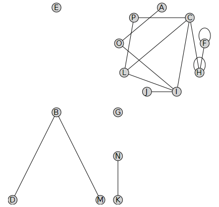
Note that there are binomial( 16, 2 ) + 16 different edges (including self-loops), so the probability of a randomly generated edge being in this graph is only about one in seven, hence not that many edges were actually deleted.
You can also use these lists to create a direct graph with a specific number of nodes; for example, this one has forty-two vertices labelled "AA" through "BP", and adds up to 100 randomly generated arcs:
[> DG := Digraph( vAA[1..42] ):
[> to 100 do
    vertex1 := vA[mod1( rand(), 16 )];
    vertex2 := vA[mod1( rand(), 16 )];
    AddArc( DG, [vertex1, vertex2] );
end do:
In a directed graph, Maple refers to connections between vertices to be arcs, while connections in an undirected graph are edges.
[> DrawGraph( DG );

Like undirected graphs, you can check if a directed graph has an edge using HasArc(...) and delete arcs using DeleteArc(...).
An edge {"A0", "B3"} can be given a weight by including the weight in a list: [{"A0", "B3"}, 3.2] where the weight is any numeric value. Similarly, [["A0", "B3"], 3.2] is used to designate the weight of the corresponding arc.
For example, the following is a weighted undirected graph:
[> WG := Graph( vA0[1..12], {[{"A0", "A4"}, 3.2],
                          [{"A2", "A7"}, 0.9],
                          [{"A2", "B1"}, 8.4],
                          [{"A3", "A9"}, 7.5],
                          [{"A4", "B1"}, 1.6],
                          [{"A5", "A7"}, 9.1],
                          [{"A6", "A9"}, 6.3],
                          [{"A7", "A6"}, 4.0],
                          [{"B0", "A1"}, 5.7],
                          [{"A8", "A2"}, 2.8],
                          [{"B0", "A2"}, 5.1]}, 'weighted' );
):
end do:
[> DrawGraph( WG );
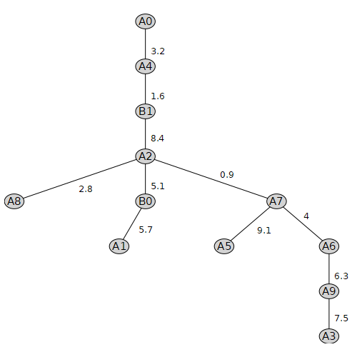
To get or set the weight of an edge, you can use the GetEdgeWeight(...) and SetEdgeWeight(...). Unfortunately, there is no corresponding GetArcWeight(...) or SetArcWeight(...). You can extract the adjacency matrix using the WeightMatrix( WG ) function.
[> WeightMatrix( WG );
$\begin{pmatrix} 0 & 0 & 0 & 0 & 3.2 & 0 & 0 & 0 & 0 & 0 & 0 & 0 \\ 0 & 0 & 0 & 0 & 0 & 0 & 0 & 0 & 0 & 0 & 5.7 & 0 \\ 0 & 0 & 0 & 0 & 0 & 0 & 0 & 0.9 & 2.8 & 0 & 5.1 & 8.4 \\ 0 & 0 & 0 & 0 & 0 & 0 & 0 & 0 & 0 & 7.5 & 0 & 0 \\ 3.2 & 0 & 0 & 0 & 0 & 0 & 0 & 0 & 0 & 0 & 0 & 1.6 \\ 0 & 0 & 0 & 0 & 0 & 0 & 0 & 9.1 & 0 & 0 & 0 & 0 \\ 0 & 0 & 0 & 0 & 0 & 0 & 0 & 4.0 & 0 & 6.3 & 0 & 0 \\ 0 & 0 & 0.9 & 0 & 0 & 9.1 & 4.0 & 0 & 0 & 0 & 0 & 0 \\ 0 & 0 & 2.8 & 0 & 0 & 0 & 0 & 0 & 0 & 0 & 0 & 0 \\ 0 & 0 & 0 & 7.5 & 0 & 0 & 6.3 & 0 & 0 & 0 & 0 & 0 \\ 0 & 5.7 & 5.1 & 0 & 0 & 0 & 0 & 0 & 0 & 0 & 0 & 0 \\ 0 & 0 & 8.4 & 0 & 1.6 & 0 & 0 & 0 & 0 & 0 & 0 & 0 \end{pmatrix}$
There are many common graphs that may be constructed without specifying each edge, and there are operations that may take one or more existing graphs and create a new graph. Some of these are listed here:
There are three sub-packages for generating specialized named graphs, random graphs, and for creating graphs based on geometric data. Commands exist to determine if a graph has specific properties, and other commands implement algorithms that traverse graphs, such as Dijkstra's algorithm. There is just so much to discuss... Enjoy.
The GraphTheory[GeometricGraphs] subpackage includes a number of commands that return graphs based on points in $\textbf{R}^n$. The first argument is either a list of $m$ lists each of $n$ entries, or it is an $m \times n$ matrix. In either case, the first index identifies the points, while the second identifies the coordinate within the point.
The algorithms are as follows: