The inttrans (integral transformation) package contains a number of functions, but engineers are generally only interested in two pairs of these: the Laplace transform and its inverse, and the Fourier transform and its inverse.
[> inttrans[laplace]( exp(-t), t, s );
$\frac{1}{s + 1}$
The second argument is the time variable, and the second is the complex frequency variable, generally $t$ and $s$, respectively. Recall that there are tables of Laplace transforms in text books, and you can replicate many of these in Maple:
[> inttrans[laplace]( u(t - 3)*exp(-t), t, s );
$\frac{e^{-3 - 3s}}{s + 1}$
In case you did not view the signal processing function page, we set u as an alias for the Heaviside function; that is, the unit step function:
[> alias( 'u' = 'Heaviside' ):
We can even try to use symbolic values:
[> inttrans[laplace]( u(t - a)*exp(-t), t, s );
$\mathcal{L}( u(t - a)e^{-t}, t, s )$
In this case, Maple cannot return a solution, because the solution depends on whether $a$ is positive or not, so we can give Maple an assumption:
[> res := inttrans[laplace]( u(t - a)*exp(-t), t, s ) assuming a >= 0;
$res := \frac{e^{-a(1 + s)}}{1 + s}$
We can now manipulate this and calculate the inverse Laplace transform:
[> inttrans[invlaplace]( res/s + 3/s + 1, t, s ) assuming a >= 0;
$-2 u(t - a) \sinh\left( -\frac{t}{2} + \frac{a}{2} \right)e^{-\frac{a}{2} - \frac{t}{2}} + 3 + \delta(t)$
If you want to use the Laplace transform on a continual basis, you may consider including the following:
[> with( inttrans ):
This loads all of the functions in the inttrans package, and we will be using these both for the Laplace transform and also for the Fourier transform in the next topic.
Going through the table of Laplace transforms found in Lathi, page 344, we have:
[> laplace( delta(t), t, s );
$1$
[> laplace( u(t), t, s );
$\frac{1}{s}$
[> laplace( t*u(t), t, s );
$\frac{1}{s^2}$
[> laplace( t^n*u(t), t, s ) assuming n >= 0;
$\Gamma(n + 1)s^{-n-1}$
In this last answer, the GAMMA(...) function is a generalization of the factorial function (the $\Gamma$ function is defined for all real numbers, while factorial is only defined for non-negative integers), and $\Gamma(n + 1) = n!$. The $\Gamma(n)$ function is undefined for integer values $0$, $-1$, $-2$, ... .
[> laplace( exp(lambda*t)*u(t), t, s );
$\frac{1}{s - \lambda}$
[> laplace( t*exp(lambda*t)*u(t), t, s );
$\frac{1}{(s - \lambda)^2}$
[> laplace( t^n*exp(lambda*t)*u(t), t, s ) assuming n >= 0;
$\Gamma(n + 1)(s - \lambda)^{-n-1}$
[> laplace( cos(b*t)*u(t), t, s );
$\frac{s}{b^2 + s^2}$
[> laplace( sin(b*t)*u(t), t, s );
$\frac{b}{b^2 + s^2}$
[> laplace( exp(-a*t)*cos(b*t)*u(t), t, s );
$\frac{s + a}{(s + a)^2 + b^2}$
[> laplace( exp(-a*t)*sin(b*t)*u(t), t, s );
$\frac{b}{(s + a)^2 + b^2}$
[> laplace( r*exp(-a*t)*cos(b*t + theta)*u(t), t, s );
$\frac{r\left(\frac{e^{j\theta}}{s - jb + a} + \frac{e^{-j\theta}}{s + jb + a}\right)}{2}$
[> laplace( exp(-a*t)*(A*cos(b*t) + (B - A*a)/sqrt(c - a^2)*sin(b*t))*u(t), t, s );
$\frac{\frac{(-Aa + B)b}{\sqrt{-a^2 + c}} + A(s + a)}{(s + a)^2 + b^2}$
Maple is aware that the Laplace transform is both linear and the effect of derivatives:
[> laplace( 3*D(y)(t) + 4*t, t, s );
$3s\mathcal{L}(y(t),t,s) - 3y(0) + \frac{4}{s^2}$
One weakness, as the one term should be $-3 \lim_{t \rightarrow 0^-} y(t)$, and not just $-3y(0)$.
Maple is also aware that the inverse Laplace transform of the product of two Laplace transforms is the convolution of the functions being transformed:
[> invlaplace( laplace(f(t)*u(t),t,s)*laplace(g(t)*u(t),t,s), s, t );
$\int_0^t f(\_U1) g(t - \_U1) d \_U1$
Note that this definition is not as careful as the convolution we previously defined. Maple also uses the rather awkward variable of integration _U1.
Now, here is an example of the power of Maple: you should be aware of the eval(...) function:
[> # Change the variable from '_U1' to 'tau'
[> eval( %, '_U1' = 'tau' );
$\int_0^t f(\_U1) g(t - \_U1) d \_U1$
You will notice that nothing happened, because the value of the integral does not depend on $_U1$. If you would prefer to see the variable of integration, you must use a differnt function: subs:
[> # Change the variable from '_U1' to 'tau'
[> subs( '_U1' = 'tau', % );
$\int_0^t f(\tau) g(t - \tau) d \tau$
This does a blind substitution of tau wherever _U1 appears. This is, however, not a mathematical evaluation, but a data structure of one variable name for another.
You can also check that specific properties are true. For example, the Laplace transform of $\frac{x(t)}{t}$ is equal to the integral of the Laplace transform of $x(t)$ integrated from $s$ to $\infty$:
[> laplace( sin(2*t)*u(t), t, s );
$\frac{2}{s^2 + 4}$
[> laplace( sin(2*t)*u(t)/t, t, s );
$\textrm{arctan}\left(\frac{2}{s}\right)$
[> int( 2/(z^2 + 4), z = s..infinity );
$-\textrm{arctan}\left(\frac{s}{2}\right) + \frac{\pi}{2}$
While at first you may not suspect that these two expressions are equal, they are, as a little bit of trigonometry will show for $s \ge 0$.
In your courses on signals and linear systems, you may have an arbitrary signal $x(t)$, and you would represent its Laplace transform as $X(s)$. It is actually possible to let Maple know about such transforms, as you may need them when you are doing, for example, work in control systems:
[> addtable( laplace, x(t), X(s), t, s );
[> addtable( laplace, y(t), Y(s), t, s );
Maple is now aware that the Laplace transform of $x(t)$ should no longer return unevaluated (as in examples above), but rather should be represented by $X(s)$.
Going through the table of Laplace transforms found in Lathi, page 369, we have:
[> laplace( x(t) + y(t), t, s );
$X(s) + Y(s)$
[> laplace( a*x(t), t, s );
$aX(s)$
[> laplace( D(x)(t), t, s );
$sX(s) - x(0)$
[> laplace( (D@@2)(x)(t), t, s );
$s^2X(s) - D(x)(0) - sx(0)$
[> laplace( (D@@3)(x)(t), t, s );
$s^3X(s) - D^{(2)}(x)(0) - sD(x)(0) - s^2 x(0)$
[> laplace( int( x(tau), tau = 0..t ), t, s );
$\frac{X(s)}{s}$
[> laplace( x(t - t0)*u(t - t0), t, s ) assuming t0 >= 0;
$e^{-s t0} X(s)$
[> laplace( x(t)*exp(s0*t), t, s );
$X(s - s0)$
[> laplace( -t*x(t), t, s );
$\frac{d}{ds} X(s)$
[> laplace( x(a*t), t, s ) assuming a >= 0;
$\frac{X\left( \frac{s}{a} \right)}{a}$
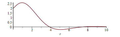
Suppose we want to solve the differential equation
$y^{(3)}(t) + 2y^{(2)}(t) + 2y^{(1)}(t) + y(t) = x^{(1)}(t) + x(t)$
subject to $x(t) = e^{-3t}u(t)$ with the inital condtions $y(0^-) = 2$, $y^{(1)}(0^-) = 1$ and $y^{(2)}(0^-) = -0.5$, so at $(0, 2)$, the solution has a slope of $1$ and a downward concavity of $-0.5$.
We will proceed as follows:
[> Id := ()  -> args:
[> x  := (t) -> exp(-3*t)*u(t):
We now proceed by describing the differential equation in Maple and finding the Laplace transform:
[> eqn := laplace( (D@@3 + 2*D@@2 + 2*D + Id)(y)(t) = (D + Id)(x)(t), t, s );
$eqn := -D^{(2)}(y)(0) + Y(s)(s + 1)(s^2 + s + 1) - y(0)(s^2 + 2s + 2) - D(y)(0)(2 + s) = \frac{s + 1}{s + 3}$
We now evaluate this Laplace transform at the initial conditions:
[> eqn := eval( eqn, [y(0) = 2, D(y)(0) = 1, (D@@2)(y)(0) = -1/2] );
$eqn := -\frac{11}{2} + Y(s)(s + 1)(s^2 + s + 1) - 2s^2 - 5s = \frac{s + 1}{s + 3}$
We will now solve this equation for $Y(s)$, the Laplace transform of $y(t)$, and we will assign to $Y$ a function mapping to this solution:
[> Y := unapply( solve( eqn, Y(s) ), s );
$Y := s \mapsto \frac{4s^3 + 22s^2 + 43s + 35}{2(s + 3)(s + 1)(s^2 + s + 1)}$
For you to find the inverse Laplace transform, you would have to convert this to a partial fraction decomposition:
[> convert( Y(s), 'parfrac' );
$\frac{-9s + 46}{14(s^2 + s + 1} + \frac{1}{7(s + 3)} + \frac{5}{2(s + 1)}$
However, we only need to request that Maple determine this inverse Laplace transform:
[> y := unapply( invlaplace( Y(s), s, t ), t )*u(t);
$y := t \mapsto \left(\frac{e^{-3t}}{7} + \frac{5e^{-t}}{2} + \frac{e^{-\frac{t}{2}}\left(101\sqrt{3} \sin\left( \frac{\sqrt{3}t}{2}\right) - 27 \cos\left( \frac{\sqrt{3}t}{2} \right)\right)}{42}\right) u(t)$
You can now plot this response:
[> plot( y(t), t = 0..10 );
Now, here is something interesting:
[> y(0);
$2$
[> D(y)(0);
$1$
[> (D@@2)(y)(0);
$\frac{1}{2}$
You'll note that this does not satisfy our initial conditions, for it is the zero-input response that satisfies the initial conditions, but note the input:
[> (D + 1)(x)(t);
$1 - 3e^{-3t}u(t) + e^{-3t}\delta(t)$
You will note the implulse function.
In the previous section, we assigned to an number of common variables, so if you would like to use these as unknowns, you can now unassign them:
[> unassign( 'x', 'y', 'Y' );