
Figure 1. A plot of four points with an interpolating cubic polynomial.
Given $n$ points of the form $(x_k, y_k)$ where all the $x$-values are different, then there is a unique polynomial of degree $n - 1$ that passes through these points.
The PolynomialInterpolation(...) function can find these points.
The points $(x_k, y_k)$ are passed as either:
For example, the following are two ways of specifying the same data:
[> xs := [3.926, 4.711, 7.364, 8.470]:
[> ys := [0.786, 1.241, 4.743, 7.207]:
and
[> xys := [[3.926, 0.786], [4.711, 1.241], [7.364, 4.743], [8.470, 7.207]]:
The next argument is the independent variable of the interpolating polynomial, or a value at which the interpolating polynomial is to be evaluated at. In almost all cases, this will be a symbol.
The points can be either numeric or algebraic expressions, which leads to some interesting properties that can be discovered.
You can either use CurveFitting['PolynomialInterpolation'](...), or you can include the CurveFitting package, and then just use the PolynomialInterpolation(...) function. We will use the first for some examples, and then look at some packages after we have included the package.
[> CurveFitting[PolynomialInterpolation]( xs, ys, x );
$0.005755330070 x^3 + 0.1232659278 x^2 - 0.8079177158 x + 1.709654479$
[> interpn := CurveFitting[PolynomialInterpolation]( xys, x );
$interpn := 0.005755330070 x^3 + 0.1232659278 x^2 - 0.8079177158 x + 1.709654479$
We can now plot both the points and the interpolating cubic:
[> plots[display](
    plots[pointplot]( xs, ys, 'symbol' = 'circle' ),
    plot( interpn, x = 3..9 )
);
Figure 1. A plot of four points with an interpolating cubic polynomial.
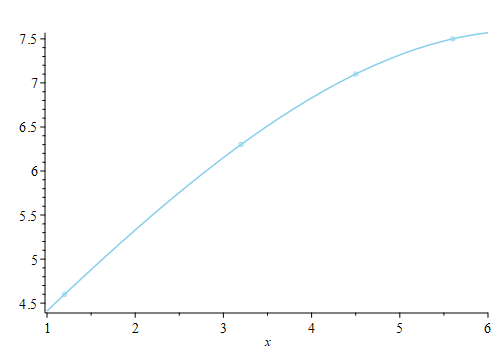
Here is another example:
[> xs := [3.2, 4.5, 1.2, 5.6]:
[> ys := [6.3, 7.1, 4.6, 7.5]:
[> interpn := CurveFitting['PolynomialInterpolation']( xs, ys, x );
$interpn := -0.007681712207x^3 - 0.00272833241x^2 + 0.9812248359x + 3.439732995$
DO NOT use polynomial interpolation if there is any significant source of noise in the data, and it is better for the $x$-values to be approximately equally spaced. Polynomial interpolation is reasonbly well suited if a sensor is being sampled periodically in the absense of significant noise.
We can plot both the points and the interpolating polynomial:
[> plots[display](
   plots['pointplot']( xs, ys, 'color' = "SkyBlue", 'symbol' = 'circle' ),
   plot( interpn, x = 1..6, 'color' = "SkyBlue" ),
   'scaling' = 'constrained'
);
Now, the polynomial interpolation described previously can easily be done in a numeric environment, and there are tools to find such interpolating polynomials quickly, so where does Maple come in? Symbolics, of course. In general, many engineering devices (e.g., sensosrs) are sampled periodically, and from that periodic sampling, it would be useful to extract additional information.
For example, suppose your deployed device is periodically sampling a voltage and you would like to estimate the rate of change of voltage at the most recent sample. Thus, our points are
$(t_0 - 2h, y(t_0 - 2h)), (t_0 - h, y(t_0 - h)), (t_0, y(t_0))$
Note that we use $t_0 - 2h$, $t_0 -h$ and $t_0$, and not three arbitrary points, as the critical point here is that the points are equalyl spaced. We can find the interpolating polynomial between these points:
[> with( CurveFitting ): # Include the CurveFitting package
[> ts := [t0 - 2*h, t0 - h, t0]:
[> map( y, ts );
$[y(t0 - 2h), y(t0 - h), y(t0)]$
[> interpn := PolynomialInterpolation( ts, map( y, ts ), t );
$interpn := \frac{\left(y \left(\mathit{t0} \right)-2 y \left(\mathit{t0} -h \right)+y \left(\mathit{t0} -2 h \right)\right) t^{2}}{2 h^{2}} $ $+\frac{\left(3 y \left(\mathit{t0} \right) h -2 y \left(\mathit{t0} \right) \mathit{t0} -4 y \left(\mathit{t0} -h \right) h +4 y \left(\mathit{t0} -h \right) \mathit{t0} +y \left(\mathit{t0} -2 h \right) h -2 y \left(\mathit{t0} -2 h \right) \mathit{t0} \right) t}{2 h^{2}}$ $+\frac{2 y \left(\mathit{t0} \right) h^{2}-3 y \left(\mathit{t0} \right) h \mathit{t0} +y \left(\mathit{t0} \right) \mathit{t0}^{2}+4 y \left(\mathit{t0} -h \right) h \mathit{t0} -2 y \left(\mathit{t0} -h \right) \mathit{t0}^{2}-y \left(\mathit{t0} -2 h \right) h \mathit{t0} +y \left(\mathit{t0} -2 h \right) \mathit{t0}^{2}}{2 h^{2}}$ $\frac{\left(y \left(\mathit{t0} \right)-2 y \left(\mathit{t0} -h \right)+y \left(\mathit{t0} -2 h \right)\right) t^{2}}{2 h^{2}}$ $+\frac{\left(3 y \left(\mathit{t0} \right) h -2 y \left(\mathit{t0} \right) \mathit{t0} -4 y \left(\mathit{t0} -h \right) h +4 y \left(\mathit{t0} -h \right) \mathit{t0} +y \left(\mathit{t0} -2 h \right) h -2 y \left(\mathit{t0} -2 h \right) \mathit{t0} \right) t}{2 h^{2}}$ $+\frac{2 y \left(\mathit{t0} \right) h^{2}-3 y \left(\mathit{t0} \right) h \mathit{t0} +y \left(\mathit{t0} \right) \mathit{t0}^{2}+4 y \left(\mathit{t0} -h \right) h \mathit{t0} -2 y \left(\mathit{t0} -h \right) \mathit{t0}^{2}-y \left(\mathit{t0} -2 h \right) h \mathit{t0} +y \left(\mathit{t0} -2 h \right) \mathit{t0}^{2}}{2 h^{2}} $
This is formula that describes the interpolating polynomial, but fortunately, we can simplify this expression:
[> interpn := simplify( interpn, 'size' );
$interpn := \frac{\left(t -\mathit{t0} \right) \left(t +h -\mathit{t0} \right) y \left(\mathit{t0} -2 h \right)+2 \left(\left(-2 t +2 \mathit{t0} \right) y \left(\mathit{t0} -h \right)+y \left(\mathit{t0} \right) \left(t +h -\mathit{t0} \right)\right) \left(\frac{t}{2}-\frac{\mathit{t0}}{2}+h \right)}{2 h^{2}}$
Important: this is the polynomial in $t$ such that if you evaluate this polynomial at the three points $t_0$, $t_0 - h$ and $t_0 - 2h$, you get the three values $y(t_0$), $y(t_0 - h)$ and $y(t_0 - 2h)$, respectively; for example,
[> eval( interpn, t = t0 - h );
$y(t0 - h)$
We can differentiate this polyninomal with respect to $t$:
[> dinterpn := simplify( diff( interpn, t ), 'size' );
$dinterp := \frac{\left(h +2 t -2 \mathit{t0} \right) y \left(\mathit{t0} -2 h \right)+\left(-4 h -4 t +4 \mathit{t0} \right) y \left(\mathit{t0} -h \right)+3 y \left(\mathit{t0} \right) \left(h +\frac{2 t}{3}-\frac{2 \mathit{t0}}{3}\right)}{2 h^{2}}$
We will now evaluate this formula at $t = t_0$:
[> simplify( eval( dinterpn, t = t0 ), 'size' );
$dinterp := \frac{3 y \left(\mathit{t0} \right)-4 y \left(\mathit{t0} -h \right)+y \left(\mathit{t0} -2 h \right)}{2 h}$
Okay, so this is the backward divided-difference formula for approximating the derivative, and this is found in most numerical methods text books together with the more familiar centered divided-difference formula:
$dinterp := \frac{y \left(\mathit{t0} + h \right)-y \left(\mathit{t0} - h \right)}{2 h}$
So how could we use Maple to find a formula we are not aware of?
Consider the following scenario: there are techniques for determining outliers, so for example, we may know that the most recent sensor reading is invalid, but we would still like to estimate the derivative at the most recent time. We cannot use the above formula on the last three points, because it would estimate the derivative one time step into the past. Instead, we can find the polynomial interpolating the points
$(t_0 - 3h, y(t_0 - 3h)), (t_0 - 2h, y(t_0 - 2h)), (t_0 - h, y(t_0 - h))$
and then differenatiate and then evaluate this interpolating polynomial at $t = t_0$:
[> ts := [t0 - 3*h, t0 - 2*h, t0 - h]:
[> simplify( eval(
    diff( PolynomialInterpolation( ts, map( y, ts ), t ), t ),
    t = t0
), 'size' );
$\frac{5 y \left(\mathit{t0} -h \right)-8 y \left(\mathit{t0} -2 h \right)+3 y \left(\mathit{t0} -3 h \right)}{2 h}$
Similarly, suppose we are now one time step into the future, but would still like to estimate the rate of change at the current time, but now the second-most recent reading is invalid, so we use the points
$(t_0 - 3h, y(t_0 - 3h)), (t_0 - 2h, y(t_0 - 2h)), (t_0, y(t_0))$
recalling that $y(t_0 - h)$ is an invalid reading, so we have:
[> ts := [t0 - 3*h, t0 - 2*h, t0]:
[> simplify( eval(
    diff( PolynomialInterpolation( ts, map( y, ts ), t ), t ),
    t = t0
), 'size' );
$\frac{5 y \left(\mathit{t0} \right)-9 y \left(\mathit{t0} -2 h \right)+4 y \left(\mathit{t0} -3 h \right)}{6 h}$
These are formulas usually not found in text books, but can easily be derived using Maple, and are potentially useful in specific real-world applications. You can, of course, derive similar formulas for accelleration and integrals:
[> ts := [t0 - 3*h, t0 - 2*h, t0]:
[> simplify( int(
    PolynomialInterpolation( ts, map( y, ts ), t ),
    t = t0 - h..t0
), 'size' );
$\frac{h \left(21 y \left(\mathit{t0} -2 h \right)-8 y \left(\mathit{t0} -3 h \right)+23 y \left(\mathit{t0} \right)\right)}{36}$
This calculates the area under the interpolating quadratic over the most-recent time interval $[t_0 - h, t0]$, assuming the second-most recent reading, that at $t_0 - h$, is not available.
These are formulas usually not found in text books, but can easily be derived using Maple, and are potentially useful in specific real-world applications. You can, of course, derive similar formulas for accelleration and integrals: