An initial value problem is a first-order ordinary differential equation
together with an initial condition
We will assume that the differential equation can be written in the above form, which is true in many cases in practice.
We are trying to find a function y(t), the derivative of which satisfies the first equation, and when we evaluate the function at t0, it evaluates to y0.
We know that a continuous function can be approximated by a straight line, at least, locally, so if we have the slope of the function (it's given to us by the equation y(1)(t) = f(t, y(t)) ), why not approximate the function by this line. The equation of this line is y0 + f(t0, y0) (t - t0)
Therefore, if we want to approximate y(t1), we can just evaluate the straight line to get:
If we denote h = t1 − t0, then this simplifies to:
We will denote this approximation by y1.
Graphical Representation
To visualize this, consider the first-order ODE
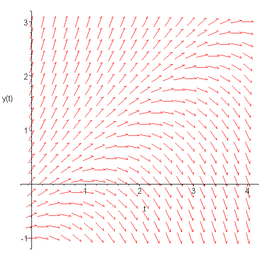
Let's pick a 21 × 21 grid of points on (t, y) ∈ [0, 4] × [-1, 3] and evaluate the slope at those points. Next, plot an arrow with the slope at that point. This is shown in Figure 1.

Figure 1. The slopes defined by the given ODE for various values of t and y.
Thus, a solution which passes through (or close to) one of the given points must have a slope equal to (or close to) the slope of the arrow.

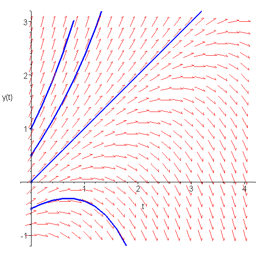
Figure 2. Four solutions given four different initial conditions.
You can almost draw the solutions in by hand, simply by following the arrows. Figure 2 shows four separate initial conditions: y(0) = -0.5, y(0) = 0, y(0) = 0.5, and y(0) = 1. Note how each solution has, in all cases, a slope which closely matches any arrows which it may pass?
Example
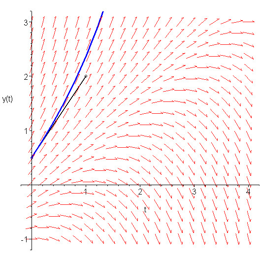
Thus, suppose we start with the initial condition y(0) = 0.5. If we want to approximate y(1) for the solution which has the initial condition y(0) = 0.5, why not follow the slope at (0, 0.5) out a distance 1. This is demonstrated in Figure 3.

Figure 3. Approximating y(1) using the initial condition y(0) = 0.5 and the slope at that point.
This gives us an approximate value of y(1) ≈ 0.5 + 1.5⋅1 = 2.
We can find (using calculus) that the actual solution is y(t) = t + ½et. First, we note that y(0) = 0 + ½e0 = 0.5, and thus this function satisfies the initial condition, but also, if we differentiate it, we get that y(1)(t) = 1 + ½et. If we rewrite this as y(1)(t) = 1 − t + (t ½et), we note that the object in the brackets is y(t), and therefore y(1)(t) = 1 − t + y(t), which is the differential equation we started with.
Therefore, the approximation y(1) ≈ 2 is not close, but is not unreasonably far from the correct answer of 2.35914.
Copyright ©2005 by Douglas Wilhelm Harder. All rights reserved.


