Introduction Notes Theory HOWTO Examples Engineering Error Questions Matlab Maple

The multiple-step 4th-order Runge Kutta lacks flexibility. In order to determine if a step size of h is neither too large nor too small, it is necessary to find the solution with a smaller step size, say h/2 and to test if the differences in the y values corresponding to the same t values are sufficiently close.

Presented is an alternate Runge Kutta technique which uses two separate calculations to determine if the step size is sufficiently small and we can modify the size of the step as appropriate. Such a technique is known as adaptive.

I'd like to thank Allan Wittkopf for his suggestions and help.

Background

Useful background for this topic includes:

14.3 4th-Order Runge Kutta Method

References

Bradie, Section 7.7, Error Control and Variable Step Size Algorithms, p.609.
Mathews, Section 9.5, Runge-Kutta Methods, p.497.

Theory

Recall how with Richardson Extrapolation, we found two approximations, for example, R_,0 and R_1,0. We used the property that the error reduces by O(h²) to define R_1,1 as a linear combination of the first two approximations in such a way that the error was canceled, resulting in an answer which was O(h⁴).

Unfortunately, we cannot come up with a method which works as simply as this for IVPs. Instead, however, we will do is use an b(h²) method, and then use and b(h³) method to approximate the error for the b(h²) method, allowing us to determine if the value of h is sufficiently small.

This document is divided into two sections:

A simple example showing how Heun's method can be used to determine if h is sufficiently small so that Euler's method is sufficiently accurate.
Next we will look at the Runge-Kutta-Fehlberg method which uses b(h⁴) and b(h⁵) methods.

Unfortunately, there are some controversies surrounding the application of the Runge-Kutta-Fehlberg method.

Euler and Heun

Consider the IVP

y⁽¹⁾(t) = ½ y(t) - t + 1
y(0) = 0.5

If we use both Euler's method and Heun's method to approximate y(0.1), we get:

y₁ = 0.625
z₁ = 0.62125

If we calculate the difference, we get we get y₁ − z₁ = 0.001875. The error of y₁ is y₁ − y(0.1) = 0.001907. You will note that the difference between Heun's method and Euler's method is, in this case, a good approximation to the error of Euler's method. To examine why this is true, consider the following reasoning:

The Taylor series approximations for these two approximations are:

and

Subtracting the first equation from the second yields:

If the h³ is sufficiently small, the third term is negligible, and therefore, we have:

Notice that this is now a good approximation to the error for y₁, and, for sufficiently small h, if we want to ensure that the error is less than some fixed value ε_abs, we can find the optimal step size sh by realizing that

|z₁ - y₁| ≈ ½f⁽²⁾(τ) h².

We want to find that multiple sh such that

½f⁽²⁾(τ) (sh)² = ε_abs.

By equating these two equations and solving for s, we get that:

This technique does not give us any idea as to how good our approximation with Huen's method is, it only gives us a reasonable estimate as to the error of Euler's method. Thus, we should determine the optimal h value to use and then use the corresponding Euler approximation.

Example

Consider the IVP:

y⁽¹⁾(t) = 2 y²(t) - t² + 1
y(1) = 1

This differential equation has no simple solution, however, suppose we start with a value of h = 0.1 but we want to ensure that the error is approximately ε_abs < 0.001.

To solve this, we find the approximations:

K₀ = f( t₀, y₀ )
y₁ = y₀ + h K₀
K₁ = f( t₁, y₁ )
z₁ = y₀ + ½ h (K₀ + K₁)

that is,

K₀ = f( 1, 1 ) = 2
y₁ = 1 + 0.1⋅2 = 1.2
K₁ = f( 1.1, 1.2 ) = 2.67
z₁ = 1 + ½ 0.1 (2 + 2.67) = 1.2335

The actual value of the solution is y(1.1) = 1.23785803, and thus, the absolute error of Euler's approximation (the first) is 0.03785803 which is significantly larger than the acceptable error 0.001.

Thus, the optimal value of h may be found by calculating

s = (0.001 / |1.2335 - 1.2|)^½ = (0.001/0.0335)^½ ≈ 0.173

Thus, we should use h = hs = 0.1⋅0.173 = 0.0173. If we do, we get:

y₁ = y₀ + h*f(t₀, y₀) = 1 + 0.0173 f(1, 1) = 1.0346

and the correct value is y(1.0173) = 1.035531805 and thus, the absolute error is now 0.0009318 which is very close to the desired error of 0.001.

Runge Kutta Fehlberg

Unfortunately, Euler's method is not very efficient, being an O(h) method if are using it over multiple steps. Because Heun's method is O(h²), it is referred to as an order 1-2 method.

The Runge-Kutta-Fehlberg method uses an O(h⁴) method together with an O(h⁵) method and hence is often referred to as RKF45.

Thus, we are sampling:

the slope K₁ at the point (t₀, y₀),
the slope K₂ at t₀ + 1/4 h following the slope K₁,
the slope K₃ at t₀ + 3/8 h following a linear combination of the slopes K₁ and K₂,
the slope K₄ at t₀ + 12/13 h following a linear combination of the slopes K₁ through K₃,
the slope K₅ at t₀ + h following a linear combination of the slopes K₁ through K₄, and
the slope K₆ at t₀ + 1/2 h following a linear combination of the slopes K₁ through K₅.

With these six approximations of the slope, we notice that the sum of the linear combinations is, in all cases, one:

1/4 + 3/4 = 1
161/169 − 600/169 + 608/169 = 1
8341/4104 − 32832/4104 + 29440/4104 − 845/4104 = 1
−6080/10260 + 41040/10260 − 28352/10260 + 9295/10260 − 5643/10260 = 1

After this, the linear combination is multiplied by the step size times h.

Thus, each linear combination of slopes is an estimator of the actual slope.

The next insight was write two formulae for the approximate the value at t₁:

and

Note that in each case, the sum of the coefficients of the terms in the numerator equals the denominator, so once again, each is an unbiased estimator of the slope.

It can be shown that the first formula is an O(h⁵) while the second is O(h⁶) (though only O(h⁴) and O(h⁵), respectively, if multiple steps are used). As in the example above, we can use these two solutions to estimate the appropriate size of sh to ensure that the error is close tot ε_abs:

Multiple Steps

The most naive application of either of these adaptive techniques is to start with h = h₀ for some initial value of h₀. Next, given (t_k, y_k), use the current value h to calculate the value of s, assign h = sh and use this new value of h to approximate (t_k + 1, y_k + 1).

Maximum and Minimum Sizes for h

The first thing we must guard against is an accidental increase in h which is too large and consequently yields an incorrect result. Thus, it is usual to define some maximum value h_max. Similarly, it may be too expensive to have h too small, and therefore, we set a minimum value h_min.

Irrational Step Size

The step size is going to be irrational, as in both cases, we are calculating either a square or 4th root. Consequently, each of the step sizes will be different. One solution to this is to allow the step size to be of the form 2ⁿh₀ where h₀ is the initial step size and n is restricted to some range [-N, N] (this solves the previous problem.

Use The First Approximation

If s has been calculated and found to be greater than 1, then use the approximation of y_{k + 1} which was used to find s.

Do NOT use the Higher-Order Approximation

One obvious observation is that, if we have calculated both y_{k + 1} and z_{k + 1}, why not use the second (higher-order) approximation. Unfortunately, the error analysis was performed for the first, and therefore, if the goal is to have the error set by some bound, use y_{k + 1}. The error of the z approximation is unknown.

Many textbooks will use z, and this will be completely fine for nice IVPs, however, if the ODE is stiff (as we will see in the next topic), using the z term will be seen to be sub-optimal.

Example

The following example shows how we can solve the following IVP using the techniques explained above and observe some of the problems mentioned above.

Suppose we have the IVP

y⁽¹⁾(t) = -2y(t) + e^{-2(t - 6)²}
y(0) = 1

The solution to this differential equation is initially a curve which decays exponentially, followed by a pulse around time t = 6, followed again by an exponentially decaying curve. The solution is shown in Figure 1 on the interval [, 10].

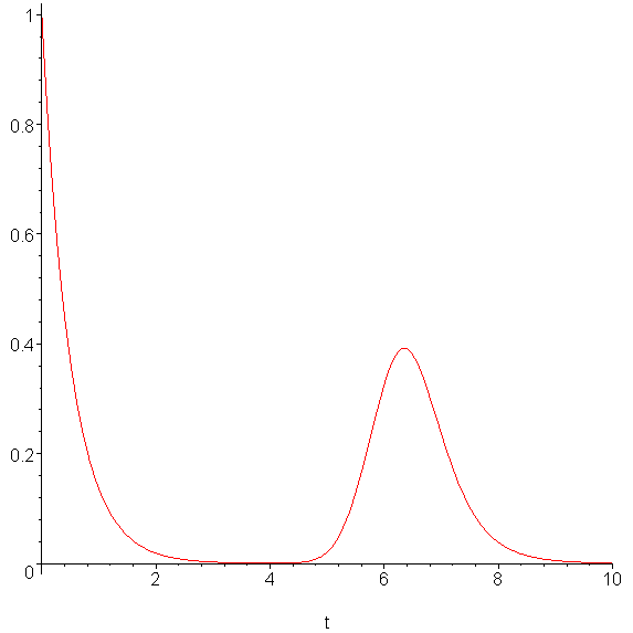
Figure 1. The solution to the given IVP.

If we use Euler's method using h = 0.05, then we need 200 steps to approximate the solution. Approximation is shown in Figure 2 and the error at each point is shown in Figure 3.

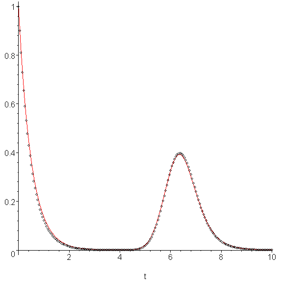
Figure 2. Multiple steps of Euler's method using h = 0.05.

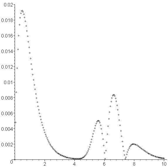
Figure 3. The errors at each of the 200 points.

We note that the error does not go above 0.02.

If we use the Euler-Heun method described above at each step, always using the optimal value of h, we get the approximation shown in Figure 4, the errors being shown in Figure 5.

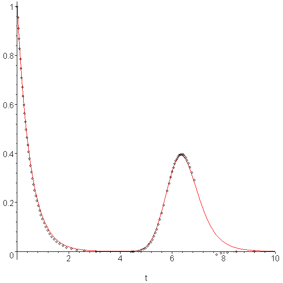
Figure 4. Using the adaptive Euler-Heun method with ε_abs = 0.01.

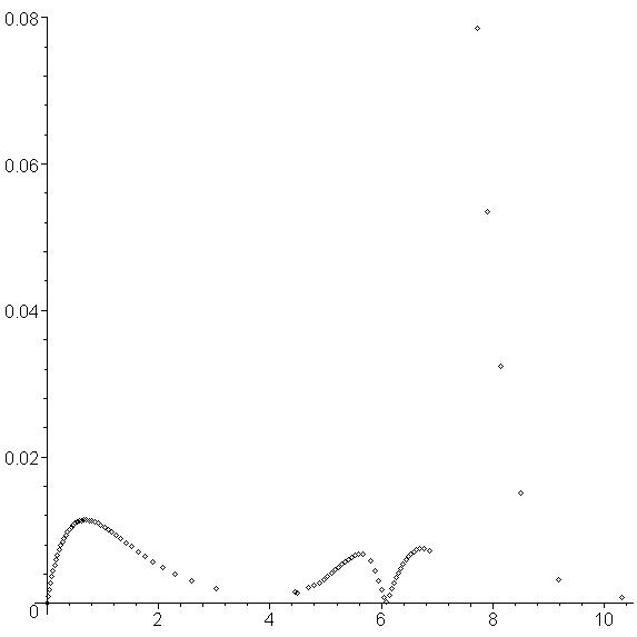
Figure 5. The errors associated with the adaptive Euler-Heun method.

This required 82 iterations of the technique before the value of t₈₂ = 10.3097 ≥ 1, or half as many points. On the first trough, it is quite apparent that the size of h quite large, however, after the second peak, we also note that the value of h was too large, and therefore the next step was negative. Before that point, the error never went above 0.012, which is significantly better than using Euler's method with h = 0.05 (this method having a maximum absolute error closer to 0.02). Also, looking at the first ten t values, we see that they are unevenly spaced:

0, 0.02236067977, 0.04523878102, 0.06865896511, 0.09264770682, 0.1172334795

If, instead, we adopt some of the suggestions above for multiple step methods, where we:

Start with h = 0.1,
Double h if s ≥ 1.5, up to a maximum of 0.4, but use the y used to approximate s, and
Halve h if s ≤ 0.75 down to a minimum of 0.25 and use the new value of h.

The result is an approximation to the solution using 104 points (instead of 200) and this is shown in Figure 6. The errors are shown in Figure 7, and it can be quite easily observed that the errors are significantly less then using an unmodified Euler's method with h = 0.05, even though we use a minimum h value of 0.025. The jump sizes are shown in Figure 8.

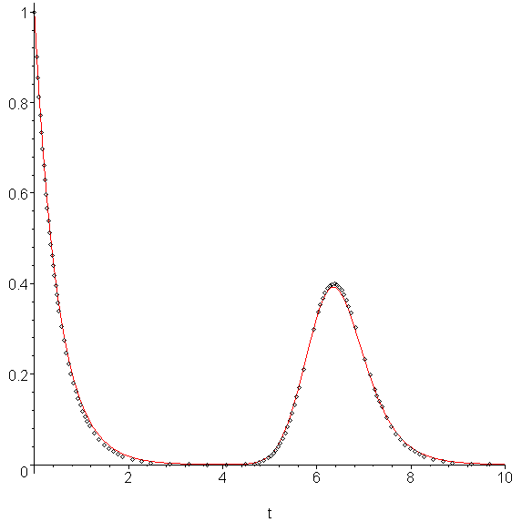
Figure 6. Using a modified adaptive Euler-Heun method with ε_abs = 0.01.

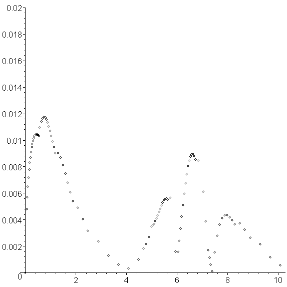
Figure 7. The errors associated with the modified adaptive Euler-Heun method.

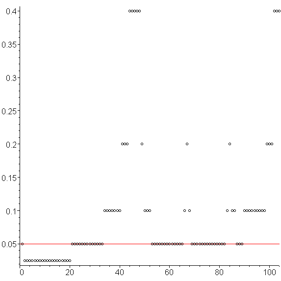
Figure 8. The step sizes used with the modified adaptive Euler-Heun method.

The points at which approximations are found are:

0, 0.05, 0.075, 0.1, 0.125, 0.15, 0.175, 0.2, 0.225, 0.25, 0.275, 0.3, 0.325, 0.35, 0.375, 0.4, 0.425, 0.45, 0.475, 0.5, 0.525, 0.575, 0.625, 0.675, 0.725, 0.775, 0.825, 0.875, 0.925, 0.975,
1.025, 1.075, 1.125, 1.175, 1.275, 1.375, 1.475, 1.575, 1.675, 1.775, 1.875,
2.075, 2.275, 2.475, 2.875,
3.275, 3.675,
4.075, 4.475, 4.675, 4.775, 4.875, 4.975,
5.025, 5.075, 5.125, 5.175, 5.225, 5.275, 5.325, 5.375, 5.425, 5.475, 5.525, 5.575, 5.625, 5.725, 5.925,
6.025, 6.075, 6.125, 6.175, 6.225, 6.275, 6.325, 6.375, 6.425, 6.475, 6.525, 6.575, 6.625, 6.675, 6.725, 6.825,
7.025, 7.125, 7.225, 7.275, 7.325, 7.375, 7.475, 7.575, 7.675, 7.775, 7.875, 7.975,
8.075, 8.175, 8.275, 8.475, 8.675, 8.875,
9.275, 9.675,
10.075

and it is therefore obvious that most of the approximations are used to fit the curve on the intervals [0, 2] and at the start, middle, and end of the peak.

To conclude, we will also show the affect of using the default RKF45 method which always uses the optimal h value to approximate the solution on the interval, we reduce the number of points required to 16, as is shown in Figure 9. The errors are shown in Figure 10, and the step sizes are shown in Figure 11. The red line shows the h = 0.025 value used above. Note that the step size grows almost to size 1. Also, because fewer steps are taken, there is a significant reduction in accumulated errors.

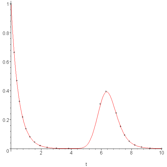
Figure 9. Using the Runge-Kutta-Fehlberg method with ε_abs = 0.01.

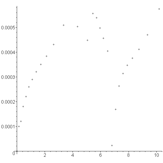
Figure 10. The errors associated with the Runge-Kutta-Fehlberg method.

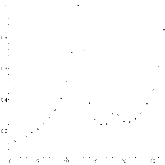
Figure 11. The step sizes used with the Runge-Kutta-Fehlberg method.

The points are:

0, 0.27282, 0.63613, 1.0650, 1.5887, 2.2509, 3.1137, 4.1975, 4.9416, 5.6021, 6.1579, 6.6112, 7.0857, 7.7649, 8.3529, 9.1176, 10.1089

If, like before, we restrict the size of h to powers of two multiplied by the default step size, we get the results shown in Figures 12 through 14. This requires 18 points, as opposed to 16.

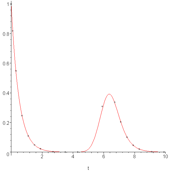
Figure 12. Using the modified Runge-Kutta-Fehlberg method with ε_abs = 0.01.

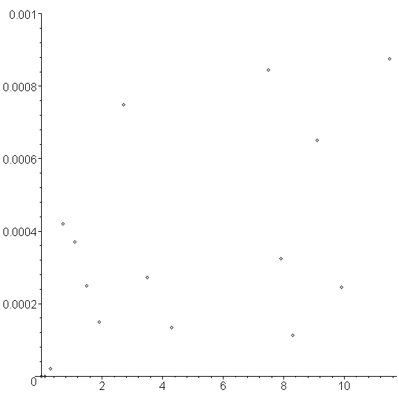
Figure 13. The errors associated with the modified Runge-Kutta-Fehlberg method.

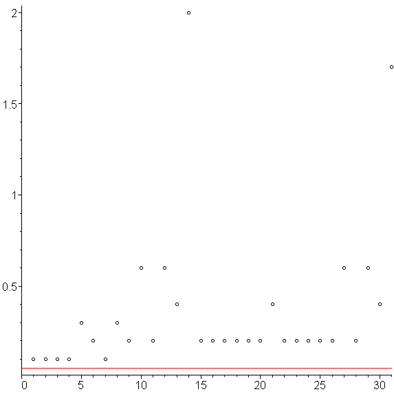
Figure 14. The step sizes used with the modified Runge-Kutta-Fehlberg method.

The points at which we approximate the solution are:

0, 0.1, 0.3, 0.7, 1.1, 1.5, 1.9, 2.7, 3.5, 4.3, 5.9, 6.7, 7.1, 7.5, 7.9, 8.3, 9.1, 9.9, 11.5

HOWTO

Problem

Given the IVP

y⁽¹⁾(t) = f( t, y(t) )
y(a) = y₀

approximate y(t) with an error less than ε_abs.

Assumptions

The function f(t, y) should be continuous in both variables.

Tools

We will use a variation of the Runge-Kutta-Fehlberg method to find two approximations of the value y(t₁) to find an optimal value of h.

Initial Conditions

Set h = t₁ − t₀. Let y₁ be the approximation of y(t₁).

Process

Define

K₀ = f( y₀, t₀ )
K₁ = f( y₀ + ½ h K₀, t₀ + ½ h )
K₂ = f( y₀ + ½ h K₁, t₀ + ½ h )
K₃ = f( y₀ + h K₂, t₀ + h )

Then let

Examples

Example 1

Apply the modified Euler-Heun method to approximate the solution to a similar IVP as shown in the theory section but with a ½(1 - cos(t)) forcing function instead of the normal curve, i.e.,

y⁽¹⁾(t) = -2y(t) + ½(1 - cos(t))
y(0) = 1

The result is as is shown in Figure 1.

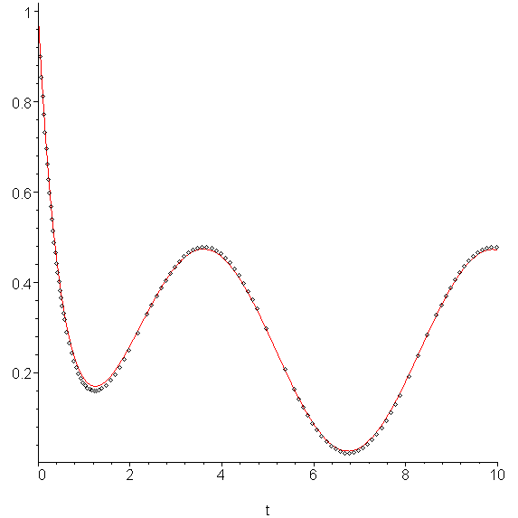
Figure 1. The approximation of the given IVP in Example 1.

Example 2

Apply the modified Runge-Kutta-Fehlberg method to the IVP described in Example 1 and list the points.

The result is as is shown in Figure 2.

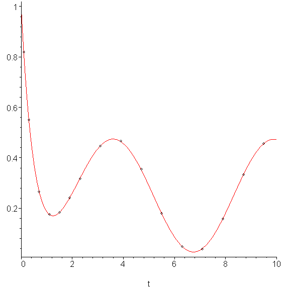
Figure 2. The approximation of the given IVP in Example 1 using RKF 45.

The t values are

0, 0.1, 0.3, 0.7, 1.1, 1.5, 1.9, 2.3, 3.1, 3.9, 4.7, 5.5, 6.3, 7.1, 7.9, 8.7, 9.5, 10.3

while the actual points are

(0.1, 0.81881)
(0.3, 0.55074)
(0.7, 0.26644)
(1.1, 0.17502)
(1.5, 0.18311)
(1.9, 0.24110)
(2.3, 0.31813)
(3.1, 0.44780)
(3.9, 0.46587)
(4.7, 0.35442)
(5.5, 0.17988)
(6.3, 0.04790)
(7.1, 0.03853)
(7.9, 0.15743)
(8.7, 0.33248)
(9.5, 0.45750)
(10.3, 0.45666)

Example 3

Approximate y(π) and y(5) using the points in Example 2.

Because π ≈ 3.1, we can probably interpolate the three points around 3.1 and evaluate the quadratic at π.

Using Matlab:

>> x = [2.3 3.1 3.9]';
>> y = [0.31813 0.44780 0.46587]';
>> poly = vander( x ) \ y
ans =

  -0.08719
   0.63290
  -0.67632

>> polyval( poly, pi )
ans = 0.45149

Because 5 is closer to the mid point between 4.7 and 5.5, it is probably best to find the interpolating cubic.

>> x = [3.9 4.7 5.5 6.3]';
>> y = [0.46587 0.35442 0.17988 0.04790]';
>> poly = vander( x ) \ y
poly =

   0.03439
  -0.53421
   2.54167
  -3.36144

>> polyval( poly, 5 )
ans = 0.29069

Example 4

Given that the actual solution to the IVP given in Example 1is the function

what is the relative error of the two values found in Example 3. Which is better and why?

From the function, we get that y(π) = (9 + 19e^-2π)/20 ≈ 0.4517740706, and therefore the relative error is 0.000629.

From the function, we get that y(5) ≈ 0.2892031203, and therefore the relative error is 0.00514.

The relative error of the first is smaller because the point π was closer to one of the actual points, namely, 3.1. As you move away from the interpolating points, the error increases.

Engineering

To be completed.

Error

The error with the Runge-Kutta-Fehlberg attempts to minimize the total error to less than ε_abs.

Questions

Question 1

Matlab

The following is an implementation in Matlab where Heun's method is used to approximate the error for Euler's method. The scaling factor is restricted to halving or doubling the size of the interval.

function [ts, ys] = heuler( f, tint, y0, h, eps_step )
    % tint is a vector of two entries represting the interval [t_0, t_end]
    t0 = tint(1);
    tend = tint(2);

    % We will start with vectors with one element and
    % continue to add further elements
    ts = t0;
    ys = y0;

    k = 1;

    while ( ts(k) < tend )
        K0 = f(ts(k), ys(k));
        K1 = f(ts(k) + h, ys(k) + h*K0);

	% Euler's approximation
        y1 = ys(k) + h*K0;

	% Heun's approximation
        z1 = ys(k) + h*(K0 + K1)/2;

        s = sqrt( eps_step/abs( y1 - z1 ) );

        if ( s < 1 )
            % h is too large
            h = h/2;
        elseif ( s < 2 )
            % h is appropriate
            ts( k + 1 ) = ts(k) + h;
            ys( k + 1 ) = y1;
            k = k + 1;
        else % s >= 2
            % h is too small
            ts( k + 1 ) = ts(k) + h;
            ys( k + 1 ) = y1;
            k = k + 1;
            h = 2*h;
        end

	% If ts(k) + h > tend, set h = tend - ts(k)
        h = min( h, tend - ts(k) );
    end
end

Maple

The Maple code for the modified Euler-Heun adaptive method is:

f := (t, y) -> -2*y + exp(-2*(t - 6)^2);
dsolve( {D(y)(t) = f( t, y(t) ), y(0) = 1} );

t[0] := 0.0;
y[0] := 1.0;
h := 0.1;
eps[abs] := 0.001;

for i from 1 do
	K[0] := f( t[i - 1], y[i - 1] );
	yt := y[i - 1] + h*K[0];

	K[1] := f( t[i - 1] + h, yt );
	zt := y[i - 1] + h*(K[0] + K[1])/2;

	s := sqrt( eps[abs] / abs( yt - zt ) );

	if s < 0.75 then
		h := max( h/2, 0.0125 );
	elif s > 1.5 then
		h := min( 2*h, 0.4 );
	end;

	t[i] := t[i - 1] + h;
	y[i] := y[i - 1] + h*K[0];

	if t[i] > 10 then
		break;
	end if;
end do:

plots[pointplot]( [seq( [t[k], y[k]], k = 1..i )] );

The Maple code for the modified Runge-Kutta-Fehlberg method is:

f := (t, y) -> -2*y + exp(-2*(t - 6)^2);
dsolve( {D(y)(t) = f( t, y(t) ), y(0) = 1} );

t[0] := 0.0;
y[0] := 1.0;
h := 0.1;
eps[abs] := 0.001;

for i from 1 do
	K[1] := f( t[i-1],             y[i-1] );
	K[2] := f( t[i-1] +   (1/4)*h, y[i-1] +   (1/4)*h*K[1] );
	K[3] := f( t[i-1] +   (3/8)*h, y[i-1] +   (3/8)*h*(        1/4*K[1] +         3/4*K[2]) );
	K[4] := f( t[i-1] + (12/13)*h, y[i-1] + (12/13)*h*(    161/169*K[1] -     600/169*K[2] +     608/169*K[3]) );
	K[5] := f( t[i-1] +         h, y[i-1] +         h*(  8341/4104*K[1] -  32832/4104*K[2] +  29440/4104*K[3] -   845/4104*K[4]) );
	K[6] := f( t[i-1] +   (1/2)*h, y[i-1] +   (1/2)*h*(-6080/10260*K[1] + 41040/10260*K[2] - 28352/10260*K[3] + 9295/10260*K[4] - 5643/10260*K[5]) );

	yt := y[i - 1] + h*(  2375*K[1] +  11264*K[3] +  10985*K[4] - 4104*K[5] )/20520;
	zt := y[i - 1] + h*( 33440*K[1] + 146432*K[3] + 142805*K[4] - 50787*K[5] + 10260*K[6] )/282150;

	s := root[4]( (eps[abs]*h)/(2*abs(yt - zt)) );

	if s < 0.75 then
		h := max( h/2, 0.025 );
		continue;
	end if;

	t[i] := t[i - 1] + h;
	y[i] := yt;

	if t[i] >= 10 then
		break;
	end if;

	if s > 1.5 then
		h := min( 2*h, 1.6 );
	end if;
end do:

plots[pointplot]( [seq( [t[k], y[k]], k = 1..i )] );

Topic 14.5: Runge Kutta Fehlberg

Background

References

Theory

Euler and Heun

Example

Runge Kutta Fehlberg

Multiple Steps

Maximum and Minimum Sizes for h

Irrational Step Size

Use The First Approximation

Do NOT use the Higher-Order Approximation

Example

HOWTO

Problem

Assumptions

Tools

Initial Conditions

Process

Examples

Example 1

Example 2

Example 3

Example 4

Engineering

Error

Questions

Question 1

Matlab

Maple