Example 1
Solve the boundary-value problem
subject to
y(1) = 2
at 9 interior points.
Using n = 10 and therefore h = 0.1, we can find:
l = 2 − 0.3 = 1.7
d = 0.16 − 4 = -3.84
u = 2 + 0.3 = 2.3
v = 0
Thus, we are solving the system
Solving this yields
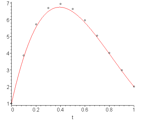
If we plot these points and the actual solution (y(t) ≈ 6.6199 e−1.5 t(2.1642 sin(2.3979 t) + 0.1511 cos(2.3979 t))) we get plot shown in Figure 1.

Figure 1. The solution to the BVP for Example 1 together with the approximation.
If we wanted a better approximation, we could use a smaller value of h.
Copyright ©2005 by Douglas Wilhelm Harder. All rights reserved.


