ECE 602 PROJECT: Operation and Configuration of Storage Portfolio via Convex Optimization

Problem formulation - Configuration Problem
Input data generation
Proposed solution
Results
Conclusions

Problem formulation - Configuration Problem

The objective of the configuration problem is to find the optimal combination of storage units to minimize the average long-term utility cost. For this purpose, the paper suggests to evaluate the long-term cost of all possible portfolio congigurations consisting of 3 storage units, being the available choices: 0,1,2 or 3 units of each type (Small S, Medium M, and Large L), Hence $$4^3$ different possible combinations. The average operational cost will be optimizing for one year which requires solving the optimal operational problem (described in the Operation.m) file every half hour for one year. In fact, from the equation of the average operational cost:

$$\mathrm{minimize\hspace{0.5cm}} \frac{1}{T} \sum_{\tau=t}^{t+T-1}\hat{p}_{\tau|t}\hat{s}_t+\alpha(\hat{r}_{\tau|t}-\hat{d}_t)_{+}$

it is implied that, the longer the period of simulation, the more exact the average operational cost is, as $$T\to\infty$ . The anual-levelized captial cost of the units are given, so the total anaul cost of the portfolio can be found as the multiplication of the number of units of each type by their respective levelized-cost. Finally, a plot of the the operational cost vs the capital cost for each possible portfolio configuraiton is presented, and the pareto optimal boundary is highlighted which can be interpretaed as the optimal solutions.

Since most of the code used to solve this problem is the same as for the operational prblem, most of the comments will be the same as in the operation.m file; however, we would like to point out that some additional code is include in this file, so additional comments have been added as well.

Input data generation

In this section, the demand and prices for a complete year of operation of the storage portfolio will be generated, using the stochastic models provided in the papaer. Likewise, some general parameters defined in the model are declared here. All these values presented have been taken directly from the original paper.

The variable Ts contains the total simulation time used to comptue the average operational cost. In this case, we will use 1 month rather than 1 year to find this value. The reason for this is that the simulation time required to solve this problem is extremely high, as highlighted by the authors of the original paper. Indeed, they use a special software to solve this problem since it can take more than 15 hours to solve it using basic solvers a CVX. Nevertheless, as we will demonstrate in the results, the differences obtained based on this asumption does not drastically affect the solution when compared to the one provided in the original paper. The reason for this is that since the cyclic behaviour of the demand remains consistent in time, i.e., does not change very much during the whole year, the value of the operational cost tends to stabilize.

Ts=2*24*30;        %Simulation time: 1 month simulations

The variable T stablishes the period for future predictions of demand and price rquired for the RHC control algorithm, i.e., 24-hours beyond "t" or 48 periods of half-hour.

T=48;                   %Period for future prediction in the RHC control

The variable Tt defines the total number of periods for which we want to forecast the price and demand. We can still forecast the demand for one year, since the computational burden for this is relatively low.

Tt=2*12*30*24;          %2 subperiods of 30 min for each hour

T_in contains the period that we will later consider as the starting point for the operatinoal problem

T_in=100;

The vectors "r" and "p" will store the actual demand and price. At every period "t" the RCH algorithm will assume that the values stored in "r" and "p" ar the historical data from which the forecast will be performed. However, "r" and "p" will be artificially generated using the procedure, also suggested in the paper.

r=zeros(Tt,1);          %Actual Request (demand)
p=zeros(Tt,1);          %Actual Price

The vector "v" will contain the optimal values of the primal varibales for the whole period of simulation

v=zeros(Tt,11);         %Vector of answers [dt st up_s1 up_s2 up_s3 um_s1 um_s2 um_s q(t+1)_s1 q(t+1)_s2 q(t+1)_s3]

The variables $$J_{op}$ and $$J_{cap}$ will store the average operational cost and captial cost of each of the portfolio alternatives.

Jop=zeros(64,1);
Jcap=zeros(64,1);

The stochastic processes of the price and demand are modeled as:

$\log(r_t)=a_r+b_r\cos(2\pi t/48 - 5\pi/4) + u_t+x_t$

$\log(p_t)=a_p+b_p\cos(2\pi t/48 - 3\pi/2) + u_t+y_t$

$u_t=hu_{t-1} + z_t$

Where $$x_t$ , $$y_t$ , and $$z_t$ are random variables normally distributed with $$\mathcal{N} (0,\sigma^2)$ . The code to set the parameters of these processes is presented below. These parameters have been taken from the original papaer.

ar=ones(Tt,1)*0.2;
br=ones(Tt,1)*0.4;
ap=ones(Tt,1)*0.15;
bp=ones(Tt,1)*0.4;
h=0.9;

The term $$u_t$ is a first order autoregressive proces. The code to generate the values of $$u_t$ is presented below

x=randn(Tt,1)*(0.01)^(1/2);
y=randn(Tt,1)*(0.01)^(1/2);
z=randn(Tt,1)*(0.01)^(1/2);
u=zeros(Tt,1);
u(1)=z(1);
    for i=2:Tt
        u(i)=h*u(i-1)+z(i);
    end

The historical values of "p" and "r" are generated using the equations presented before. The variable "t" contins the index of the total simulation time, and will be used for ploting.

t=[1:Tt]';
r=exp(ar+br.*cos(2*pi*t/T-5*pi/4)+u+x);
p=exp(ap+bp.*cos(2*pi*t/T-3*pi/2)+u+y);

The code to calculate all possible portfolio configurations is presented below

%Configuration of all possible portafolios:
opt=0:1:3;
New_D=kron(ones(1,3),opt);
Units=unique(nchoosek(New_D,3),'rows');
Units=Units+0.005;

Once all the possible portafolio configurations are found, the levelized-average cost of each is found using the code shown next.

Jcap=round(Units*[5;3;2]);

Proposed solution

In this section, the code to solve the problem will be presented. The mathematical expressions that describe the optimization problem will be commented.

The following loop is used to calculate average operational cost for each one of the 64 possible portfolio configurations.

    for k=1:64

The follwing code set the initial state of charge for each of the storage units in the portfolio

    v(T_in-1,9:11)=[Units(k,1)*2 Units(k,2)*2 Units(k,3)*1];

The loop over the variable Tau solves the optimization problem for one month (1440 periods) for the operation problem.

        for Tau=T_in:T_in+Ts

Demand and price forecast at time t

This portion of the code generates the demand and and price forcast at time=t. The forecast uses the information of the latest 24 hours (48 values) befor "t". The forecast estimate the demand and price for the next 24 hours after "t". The results are stored in two new variables: $$\hat{r_{\tau \mid t}}$ and $$\hat{p_{\tau \mid t}}$ respectively.

        r_p=r; %r_p contains the projected demand
        p_p=p; %r_p contains the projected price

The expressions used to forecast the value of the demand and price are presented below:

$\hat{r}_{\tau|t}=\mathrm{exp}(\mu_{r_{\tau|t}}+\sigma_{r_{\tau|t}}^2/2)$

$\hat{p}_{\tau|t}=\mathrm{exp}(\mu_{p_{\tau|t}}+\sigma_{p_{\tau|t}}^2/2)$

The code use to reproduce these two equations is shwon below:

            for i=1:T-1
                mean_ur=mean(log(r_p(Tau+i-T:Tau+i)));
                mean_up=mean(log(p_p(Tau+i-T:Tau+i)));
                var_ur=var(log(r_p(Tau+i-T:Tau+i)));
                var_up=var(log(p_p(Tau+i-T:Tau+i)));
                r_p(Tau+i)= exp(mean_ur+var_ur/2);
                p_p(Tau+i)= exp(mean_up+var_up/2);
            end

Optimization Problem The formulation of the convex optimization problem to solve the operational cost is presented below.

$\mathrm{minimize\hspace{0.5cm}} \frac{1}{T} \sum_{\tau=t}^{t+T-1}\hat{p}_{\tau|t}\hat{s}_t+\alpha(\hat{r}_{\tau|t}-\hat{d}_t)_{+}$

$\mathrm{subject\hspace{0.1cm}to\hspace{0.1cm}} \hat{q}_{\tau+1}=\eta^l\circ\hat{q}_{\tau}+\eta^c\circ\hat{u}_{\tau}^{+}-(1/\eta^d)\circ\hat{u}_{\tau}^{-}+\hat{w}_{\tau|t}$

$\hat{d}_{\tau}-\hat{s}_{\tau}+\textbf{1}^T u_{\tau}^{+}-\textbf{1}^T u_{\tau}^{-}=0$

$0\leq\hat{q}_{\tau}\leq Q,\hspace{0.3cm}0\leq u_{\tau}^{+}\leq C,$

$0\leq u_{\tau}\leq D,\hspace{0.3cm}\tau = t,...,t+T-1$

$\hat{q}_t=q_t, \hspace{0.3cm}\hat{q}_{t+T}=q_{final}$

$0\leq s_t \leq s_{max}$

Where:

is the number of steps in the future that the algorithm projects the price and the demand
$$\hat{p}_{\tau|t}$ is the forecasted price at time $$\tau$ based on the information available at time
$$\hat{r}_{\tau|t}$ is the forecasted demand at time $$\tau$ based on the information available at time
$$\hat{s}_{t}$ is the estimated energy purchased from the system at time
$$\hat{d}_{t}$ is the estimated energy injected into the grid at time
$$\alpha$ is the cost of the unsuplied energy
$$\hat{q}_{\tau}$ is the estimated charging level of each storage unit at time
is the actual storage level of each storage unit at time ,
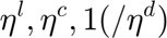$$\eta^l,\eta^c,1(/\eta^d)$ are the leakage, charging and discharging efficiencies of the storage unit respectively
$$\hat{u}_{\tau}^{+}$ and $$\hat{u}_{\tau}^{-}$ are the estimated charging and discharging rates (inflows and outflows) of the storage units at time
$$q_{final}$ is the state of charge of the portfolio at the last step of the simulation
are the unit storage capacity, maximum charging, and maximum discharging rates of the storage units respectively.
$$s_{max}$ is the maximum energy that can be purchased from the system
$$\hat{w}_{\tau|t}$ is the an additional imput of energy to the storage units. For the simulations, the authors neglect this term.

In this problem, the optimization variables are: $$\hat{d}$ , $$\hat{s}$ , $$\hat{q}$ , $$\hat{q}$ , $$\hat{u}_{\tau}^{+}$ , and $$\hat{u}_{\tau}^{-}$

As it can be seen in the problem formulation, the objective function includes two terms: the $$\hat{p}_{\tau|t}\hat{s}_t$ term represents the cost of purchasing energy at price $$s_t$ , while the term 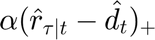$$\alpha(\hat{r}_{\tau|t}-\hat{d}_t)_{+}$ represent the cost of not supplying the demand. If the whole demand is supplied, the term $$\hat{r}_{\tau|t}-\hat{d}_t$ becomes zero; otherwise, it contains the unsupplied demand. Since the unsupplied deamnd can only be positive, the this later term has been replaced in the cost function with the variable "g" which has been declared as nonegative; hence, an additional constraint has be included in the model to defined the value of "g" as $$g=\hat{r}_{\tau|t}-\hat{d}_t$ . Furthermore, the operational cost is the devided by the total simulation time T so that an average hourly cost is found. From the convex optimization theroy, it is clear that the factor $$(1/T)$ does not affect the optimal solution.The code used to solve the optimization problem is presented below. The solver CVX has been used for this purpose.

            Smax=1.5*ones(T,1);
            alpha=20;
            ef_1=[0.98*ones(T,1) 0.99*ones(T,1) 0.995*ones(T,1)];
            ef_c=[0.8*ones(T,1) 0.9*ones(T,1) 1*ones(T,1)];
            ef_d=[(0.8)*ones(T,1) 0.9*ones(T,1) 1*ones(T,1)]; %This vector is 1/ef_d
            Q=[Units(k,1)*5*ones(T,1) Units(k,2)*2*ones(T,1) Units(k,3)*1*ones(T,1)];
            C=[Units(k,1)*0.75*ones(T,1) Units(k,2)*0.5*ones(T,1) Units(k,3)*0.5*ones(T,1)];
            D=[Units(k,1)*0.75*ones(T,1) Units(k,2)*0.5*ones(T,1) Units(k,3)*0.5*ones(T,1)];
            qfinal=[Units(k,1)*1 Units(k,2)*1 Units(k,3)*1];

            cvx_solver SDPT3
            cvx_begin quiet

            variables d(T,1) s(T,1) q(T+1,3) up(T,3) um(T,3)
            variable g(T,1) nonnegative

            minimize ((1/T)*(p_p(Tau:Tau+T-1)'*s + alpha*sum(g)))
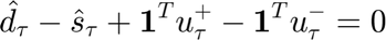
            r_p(Tau:Tau+T-1)-d==g;
            q(2:T+1,:)==q(1:T,:).*ef_1+ef_c.*up-ef_d.*um;
            d-s+up*ones(3,1)-um*ones(3,1)==0;
            zeros(T,3)<=q(1:T,:)<=Q;
            zeros(T,3)<=up<=C;
            zeros(T,3)<=um<=D;
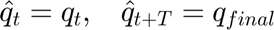
            q(1,:)==v(Tau-1,9:11);
            q(T+1,:)==qfinal;
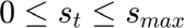
            0<=s<=Smax;

            cvx_end

The values of the parameters have been taken from the original papaer.

At every iteration, as the RCH algorithm requires, the optimal value of the state variables at time $$t$ is recorder in the vector $$v_t^*=(d_t,s_t,u_t^{+},u_t^{-})$ , while the other optimal values for the rest of the period $$t=t+1,t+2,...t+T-1$ are discared. This vector will record the optimal value of the state variables for every iteration, i.e., for every step in the whole simulation period. The code introduced to record the results is presented below.

            v(Tau,:)=[d(1,1) s(1,1) up(1,:) um(1,:) q(2,:)];

end

The following code stores the optimal operational cost of the portfolio configuration $$k$ in the vector $$Jop^k$ by plugging in the optimal variables in the objective function:

        Jop(k)=(1/Ts)*(p(T_in:T_in+Ts)'*v(T_in:T_in+Ts,2) + alpha*sum(max(r(T_in:T_in+Ts)-v(T_in:T_in+Ts,1),0)));

End of the portfolio configuration loop

end

Results

Once the operational cost has been found for all the 64 configurations, the Pareto optimal is found using the code shown below:

Opt_sol=sortrows([Jcap Jop]);

Boundary=ones(length(Opt_sol(:,1)),1);
Boundary(1)=1;
pivot=1;
c=1;

    for i=2:length(Opt_sol(:,1))
        if (Opt_sol(i,2)<=Opt_sol(pivot,2))
        pivot=i;
        c=c+1;
        Boundary(c)=i;
        end
    end

The pareto frontier stablishes configurations that cannot be improved without affecting the optimal cost (it cannot be reduced), so every point in this frontier is optimial in a multivariable optimization problem.

    All_Points_Index=[1:length(Opt_sol(:,1))]';
    Other_Points_Index = setdiff(All_Points_Index,Boundary);
    figure('Color',[1 1 1]);
    scatter(Opt_sol(Other_Points_Index,1),Opt_sol(Other_Points_Index,2));
    hold on
    scatter(Opt_sol(Boundary,1),Opt_sol(Boundary,2),'filled');
    scatter(Opt_sol(22,1),Opt_sol(22,2),'filled','MarkerEdgeColor',[0 0 0],'MarkerFaceColor',[0 0 0]);
    hold off
    xlabel('Jcap');
    ylabel('Jop');
    title('Capital cost versus average operating cost');
    axis([-inf,+inf,-inf,+inf]);

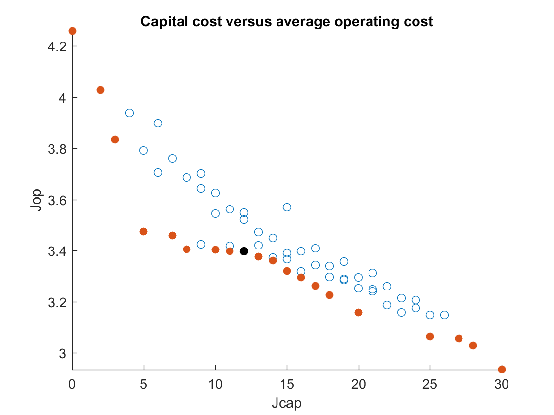
The points in red show the portafolio configurations that are part of the pareto frontier, while the other points represent the rest of configurations. The point in black is the optimal solution for the configuration presented for the the operation problem (1 small, 1 medium, and 1 large unit).

As it can be seen, the costs asociated to each option in the pareto frontier is very close to the original study as well. However, the configurations that are part of this frontier are slightly different from the original study. The reason for this is the assumption made of llenght of T (number of problmes solved to find the average oeprational cost).

Conclusions