Introduction to Optimization project:
This report replicates, analyzes and produces additional results from [1], titled: Optimal Power Control in Interference-Limited Fading Wireless Channels with Outage-Probability Specifications.
Student Names: Omar Alhussein and Ahmed Shaban.
Contents
- I: Introduction
- II-A: System model
- II-B: Problem Formulation
- II-C: Proposed solutions
- II-D: Simulation and Data Sources
- III-A: Core - Replicating the paper results
- III-B: Visualization of results in the paper
- IV-A: Incorporating the Geometric programming approach with CVX
- IV-B: Analysis of PF and CVX approaches
- V: Concluding Remarks
- VI: References
- Appendix I: Code of Perron-Frobenius Function
I: Introduction
In the assigned paper, the authors propose a power control method for interference-limited wireless networks where the fading channel is assumed to be Rayleigh distributed. The main goal is to allocate the optimal power for each transmitter/receiver (TX/RX) pair with constraints on the respective outage probability. It has been noticed that previous works (prior to 2002) focused on the signal-to-inteference (SIR) ratio, whereas this work focuses on the outage probability instead. In addition, it establishes a useful bound that relates the outage probability with the SIR when the induced multipath fading is ignored. Therewith, this allows the authors to find the optimal power not only for the original formulation but also for a lower bound with less complexity, which is favorable in wireless fading channels.
One worth mentioning caveat is that previous works assume that the power control updates are made every time the multipath fading state of the channel changes which is not practical due to the high dynamicity of fading channels. Instead the authors here incorporate the statistical variation of the Rayleigh multipath fading into account. Therefore the power control updates need to be changed at the Lognormal scale. The optimization formulations in this paper are first formulated as geometric programs (GP). Due to the high dynamicity of fading channels, using generic solvers for resultant GP formulations is not apt. Therefore, in the implementation and simulation, the authors rely the Perron-Frobenius (PF) eigenvalue theory to find the optimal power , and therefore, reduce the runtime.
In this report, we first reproduce the results from the paper, where we solve the two formulations which correspond to the optimal and lower bound solutions using the PF approach. In addition, we corraborate the aformentioned claim, where we also solve the respective problems by utilizing the relevant GP CVX solver, namely semidefinite-quadratic-linear programming (SDPT3).
II-A: System model
The authors in this paper consider an  interference channel. Each
  th transmitter sends it's message with certain power level
 . The received power at th receiver transmitted from the
  th transmitter is
  . Specifically,
  represents the distance dependant power attenuation, i.e., path loss and log-normal shadowing. It is assumed that is constant during the time scale of the analysis. On the other hand,
  captures the Rayleigh fading effect. It is assumed to be independent exponentially distributed random variable with unit mean. Therefore, the power received at receiver from transmitter is an exponentially distributed distributed random variable with mean value
  . Also, It is assumed that the interference from other transmitters is much larger than the white noise in the receiver, and thereby, it reasonable to ignore it in the analysis. Finally, the received SIR ratio at receiver is given by:
II-B: Problem Formulation
The authors consider mainly two problems of finding optimal power allocation. The first one is to find the power vector that minimizes the maximimum outage probability over all the transmitter-receiver pairs. This problem can be formulated as follows:
P1(1): Minimize 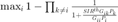
subject to 
The second problem is to maximize the certainty-equivalent margin (CEM) defined by  . This problem can be formulated as:
P2(1): Maximize 
Subject to 
II-C: Proposed solutions
First it was observed that the objective functions in both formulations are homogeneous, i.e., if  is an optimal solution then so is
  , for any
  . Here
  and
and  denote an optimal power allocation for P1 and P2 formulations, respectively. Another important observation is that the optimal solution for both problems render all outage probabilities,
  (or similarly
  )), equal. In other words,
  . With the above observations, P2 is re-written as:
P2(2): maximize 
subject to 
which can also be written as:
P2(3): minimize 
subject to:  and
and 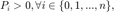
where 
Here P2(3) is solved using the PF eigenvalue theory. The largest eigenvalue in magnitude,  , along with its associated nonnegative eigenvector,
  , which is called the PF eigenvector, yeilds the optimal power allocation, i.e.,
  and
and  . Throughout our experiments, we have observed that, in our scenarios, the eigenvector corresponding with the largest eigenvalue is actually the PF vector. Therefore, there is no need to implement sophisticated algorithms to get the PF vector. However, for the sake of completeness, we have put a very effecient implementation that is based on [2] in the appendix, albeit it is not used in the simulations.
P2(3) is solved using the PF method in Section III. We also implement P2(2) using CVX in Section IV to validate that both approaches yeild the same solution and to get sense of the runtime difference.
As for P1, after few consecutive manipulations, it can be written as
P1(2): minimize 
subject to 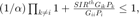 and
and 
Here the optimal outage is  . To solve this problem, The authors propose an iterative PF method. First the problem is re-written as:
P1(3): minimize
subject to 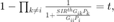 and
and
After some manipulations, the equality constraint is expressed as  , where
  is given by:
and 
The iterative PF method works as follows: (1) start with  from P2(3), (2) fix
  and update by solving the PF eigenvalue problem, and (3) repeat until P does not change a lot. The paper didn't specify a tolerance threshold. In our simulations, we used a tolerance of
  since we observed it is a very fast and accurate algorithm; it most often converges in 3-4 iterations only.
Again for P1, we first replicate the results in the paper using the iterative PF method in Section III. In Section IV, we implement the geometric program P1(2) using CVX. Note that we only replicated the results of the paper using the PF method because since the paper uses a large number of variables, and the CVX approach would take unreasonably huge time to solve P1 when the number of transmitters is n=50. Therefore, in Section IV, we compare the PF and CVX approaches with reduced number of transmitters, namely we assume assume n=5 in Section IV.
II-D: Simulation and Data Sources
The paper assumes number of transmitters/receivers n=50. As for the gain matrix G, it is assumed that  since it resembles the desired channel, i.e.,
  -->
-->  . The cross-gain interference paths are assumed to be uniformly generated random variable between 0 and 0.001. For both Sections III, we replicate the results with the preceding assumptions. In Section IV, we set n to 5 for the CVX formulation to not consume a long runtime.
III-A: Core - Replicating the paper results
Here we replicate the results of the paper using the PF eigenvalue method , namely we reproduce Figures 1 and 3.
clear; close all ; clc ; cvx_clear ;
n = 50; % number of TXs/RXs
G = 0.001*rand(n); % Gain Matrix
G = G - diag(diag(G)-1); % set diagonal to 1.
% SIR = 3:3:10; % Range of the threshold Signal-to-Interference ratio
SIR = [ 3 6 9 10];
m = length(SIR);
OLower = zeros(m,1); % Lower bound on outage probability
OOpt = zeros(m,1); % Optimal outage probability (w/ Heuristic PerronFrobenious)
CEM = zeros(m,1); % Optimal Certainty-Equivalent Margin (Heuristic PF)
delta = 10^-20  ; % Tolerance threshold for convergence
for iter = 1:m
    %================== P2(3): CEM solution w/ PF ============
    A = zeros(n);
    for i=1:n
        for j=1:n
            A(i,j) = G(i,j) ./ (SIR(iter) * G(i,i)) ;
        end
    end
    % To find the Perron vector. With extensive experiments, we observed
    % that the eigenvector, with the highest eigenvalue, is actually the
    % perron vector in this context for matrix A. Therefore, we don't
    % implement sophisticated algorithms for that. For completeness, in
    % case we have different scenario for A, we can use the function
    % Perron(A), which is attached in the appendix, but it is not used
    % here.
    %   [~,P_cem] = perron(A) ; % Here the vector is positive. (alpha * maxVector) >=0
    [e1,e2] = eig(A);
    %   [value,idx] = max(max(abs(e2))); %idx=1 always cuz of matlab, so ignore;
    P_cem = e1(:,1);
    if(sign(P_cem)==-1)
        P_cem = -P_cem;
    end
    P_cem = P_cem./sum(P_cem);


    O_lower = ones(1,n);
    for i=1:n
        for k=1:n
            if(k~=i)
                O_lower(i) = O_lower(i) * (1 + SIR(iter) * G(i,k) * P_cem(k) / (G(i,i)*P_cem(i)) )^-1 ;
            end
        end
        O_lower(i) = 1 - O_lower(i) ;
    end
    OLower(iter) = max(O_lower) ;
    cem = zeros(1,n);
    for i=1:n
        for k=1:n
            if(k~=i)
                cem(i) = cem(i) + G(i,k) * P_cem(k);
            end
        end
        cem(i) = G(i,i) * P_cem(i)./(SIR(iter)*cem(i)) ;
    end
    CEM(iter) = min(cem);
    %================== P1(3): Optimum solution w/ iterative PF ============
    %iterative perron forbienus
    B=zeros(n);
    P=P_cem;
    for q=1:10% ten iterations is more than enough(it stated in the paper that usually covergence occurs after 3 to 4 iterations)
        for i=1:n
            for j=1:n
                if(j~=i)
                    B(i,j) =(P(i)/P(j))*log(1+SIR(iter)*G(i,j)*P(j)./(G(i,i)*P(i)));
                else
                    B(i,j)=0;
                end
            end
        end
        %     [r,P] = perron(B);
        [e1,e2] = eig(B);
        [r,idx] = max(max(abs(e2))); %idx=1 always cuz of matlab, so ignore;
        %     value - r
        %     pause;
        P_temp = e1(:,1);
        if(sign(P_temp)==-1)
            P_temp = -P_temp;
        end
        P_temp = P_temp./sum(P_temp);
        P = P_temp ;
        if (sum(B*P-r*P)<delta) % to terminate when convergence occurs
            %             disp([ 'iterative PF for SIR= ' num2str(SIR(iter)) ', converged in' num2str(q) ' iterations.' ]);
            break;
        end
    end
    P_opt=P;
    O_opt = ones(1,n);
    for i=1:n
        for k=1:n
            if(k~=i)
                O_opt(i) = O_opt(i) * (1 + SIR(iter) * G(i,k) * P_opt(k) / (G(i,i)*P_opt(i)) )^-1 ;
            end
        end
        O_opt(i) = 1 - O_opt(i) ;
    end
    OOpt(iter) = max(O_opt) ;
end
III-B: Visualization of results in the paper
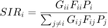
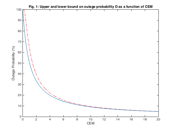
In Fig. 1, the relation between the upper and lower bound of the outage probability is plotted as a function of the CEM. The purpose was to show that the bound is in fact very tight for the outage probabilities of interest at ~20% and lower. The relation governing Fig. 1 is:
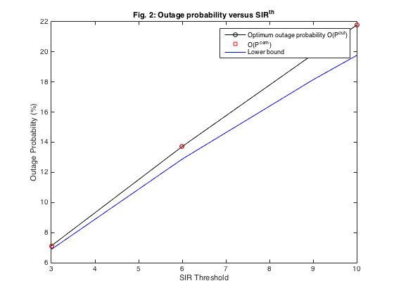
In Fig. 2, the SIR is sweeped from 3 to 10. For each SIR, we first find and . And, then we plot  ,
,  , and the lower bound
  . As seen, because the bound is actually tight, the result we obtained from P1 and P2 are, for practical purposes, equal. This implies that one doesn't need to run the iterative PF method, and simply be confined with solving P2 only.
%======== Plotting and Analysis =========================
figure; % Fig. 1 in Paper.
CEN= 0:.01:20;
Lowerbound=100*1./(1+CEN);
Upperbound=100*(1-exp(-1./CEN));
plot(CEN,Upperbound,'-. r' , CEN, Lowerbound);
ylabel('Outage Probability (%)');
xlabel('CEM');
title('Fig. 1: Upper and lower bound on outage probability O as a function of CEM');

figure; % Fig. 2 in Paper.
plot(SIR,100*OOpt,'k-o',SIR,100.*OLower,'rs',...
    SIR,100./(CEM+1),'b');
legend('Optimum outage probability O(P^{out})','O(P^{cem})','Lower bound');
ylabel('Outage Probability (%)');
xlabel('SIR Threshold');
title('Fig. 2: Outage probability versus SIR^{th}');
IV-A: Incorporating the Geometric programming approach with CVX
As mentioned before, solving the GP-based formulation with CVX requires a lot of time. Therefore, in this section, we set  to 5. The main objective is to first corraborate that our CVX approach matches the result obtained from the PF method. In addition, it would be interesting to visualize the difference between the runtime of both approaches for both the CEM maximization (P2) and optimal outage probability (P1) formulations.
clear; close all ; clc ; cvx_clear
n = 5; % number of TXs and RXs
P = zeros(n,1) ; % Transmitter powers (optimization variables)
G = 0.001*rand(n); % Gain Matrix
for i=1:n
    G(i,i) = 1 ;
end
% SIR = 3:1:10; % Range of the threshold Signal to Interference noise ratio
SIR = [ 3 6 9 10];
m = length(SIR);
OLower = zeros(m,1); % Lower bound on outage probability
OOpt = zeros(m,1); % Optimal outage probability (w/ Heuristic PerronFrobenious)
CEM = zeros(m,1); % Optimal Certainty-Equivalent Margin (Heuristic PF)
OOpt_gp = zeros(m,1); % Optimal outage probability (w/ CVX-Geometric Program)
CEM_gp = zeros(m,1); % Optimal CEM (w/ CVX-GP)
delta = 10^-20  ; % Error Threshold for convergence

CEM_toc = 0 ; % Avg time of all iterations with PF CEM.
OOpt_toc = 0 ; % Avg time of all iterations with PF Outage.
OOpt_gp_toc = 0 ; % Avg time of all iterations with GP-based outage.
CEM_gp_toc = 0 ; % Avg time of all iterations with GP-based CEM.
montee = 5; % will repeat the experiment 30 times to average the runtimes.
for idx=1:montee
    for iter = 1:m %iterating over the SIR threshold
        %================== CEM solution w/ PF ============
        tic;
        A = zeros(n);
        for i=1:n
            for j=1:n
                A(i,j) = G(i,j) ./ (SIR(iter) * G(i,i)) ;
            end
        end
        %   [~,P_cem] = perron(A) ; % Here the vector is positive. (alpha * maxVector) >=0
        [e1,e2] = eig(A);
        %   [value,idx] = max(max(abs(e2))); %idx=1 always cuz of matlab, so ignore;
        P_cem = e1(:,1);
        if(sign(P_cem)==-1)
            P_cem = -P_cem;
        end
        P_cem = P_cem./sum(P_cem);
        CEM_toc = CEM_toc + toc;
        O_lower = ones(1,n);
        for i=1:n
            for k=1:n
                if(k~=i)
                    O_lower(i) = O_lower(i) * (1 + SIR(iter) * G(i,k) * P_cem(k) / (G(i,i)*P_cem(i)) )^-1 ;
                end
            end
            O_lower(i) = 1 - O_lower(i) ;
        end
        OLower(iter) = max(O_lower) ;

        cem = zeros(1,n);
        for i=1:n
            for k=1:n
                if(k~=i)
                    cem(i) = cem(i) + G(i,k) * P_cem(k);
                end
            end
            cem(i) = G(i,i) * P_cem(i)./(SIR(iter)*cem(i)) ;
        end
        CEM(iter) = min(cem);
        %================== Optimum solution w/ iterative PF ============
        % Iterative perron forbienus
        tic;
        B=zeros(n);
        P=P_cem;
        for q=1:10
            for i=1:n
                for j=1:n
                    if(j~=i)
                        B(i,j) =(P(i)/P(j))*log(1+SIR(iter)*G(i,j)*P(j)./(G(i,i)*P(i)));
                    else
                        B(i,j)=0;
                    end
                end
            end
            %     [r,P] = perron(B);
            [e1,e2] = eig(B);
            [r,~] = max(max(abs(e2))); %idx=1 always cuz of matlab, so ignore;
            %     value - r
            %     pause;
            P_temp = e1(:,1);
            if(sign(P_temp)==-1)
                P_temp = -P_temp;
            end
            P_temp = P_temp./sum(P_temp);
            P = P_temp ;
            if (sum(B*P-r*P)<delta) % to terminate when convergence occurs
                break;
            end
        end
        OOpt_toc = OOpt_toc + toc ;
        P_opt=P;
        % Calculating the optimal outage probability
        O_opt = ones(1,n);
        for i=1:n
            for k=1:n
                if(k~=i)
                    O_opt(i) = O_opt(i) * (1 + SIR(iter) * G(i,k) * P_opt(k) / (G(i,i)*P_opt(i)) )^-1 ;
                end
            end
            O_opt(i) = 1 - O_opt(i) ;
        end
        OOpt(iter) = max(O_opt) ;

        %================== CEM solution w/ CVX ===========
        %   [CEM_gp(iter),~,CEM_temp_gp_toc] = CEM_CVX(G,SIR(iter)); %can be found in appendix
        n = size(G,1);
        G_diag = diag(G);          % main diagonal of G
        G_nodiag = G - diag(G_diag); % G matrix w/ no diagonal
        cvx_clear
        tic;
        cvx_begin gp quiet
        variables t P(n)
        minimize(t)
        subject to
        (G_diag.*P)./(SIR(iter)*G_nodiag*P) >= (1/t) .* ones(n,1) ;
        P >= zeros(n,1);
        cvx_end
        PP = P ;
        CEM_gp(iter) = t ;
        CEM_gp_toc = CEM_gp_toc + toc ;
        %     [OOpt_gp(iter),~,OOpt_temp_gp_toc] = Optimal_outage_CVX(G,SIR(iter));
        if(idx == 1 && iter == 1)
            tic;
            cvx_begin gp %quiet % note: quiet mode doesn't really reduce the timing req. of SDPT method.
            variables P(n) aa
            minimize(aa)
            subject to
            P >= zeros(n,1);
            for i=1:n
                O = 1 ;
                for j=1:n
                    if(i~=j)
                        O = O * (1+SIR(iter)*G(i,j)*P(j)/(G(i,i)*P(i))); % as product of monomials.
                    end
                end
                (1/aa)*O <= 1 ;
            end
            cvx_end
            PP = P ;
            OOpt_gp_toc = OOpt_gp_toc + toc;
            OOpt_gp(iter) = 1-1/aa;
        else
            tic;
            cvx_begin gp quiet % note: quiet mode doesn't really reduce the timing req. of SDPT method.
            variables P(n) aa
            minimize(aa)
            subject to
            P >= zeros(n,1);
            for i=1:n
                O = 1 ;
                for j=1:n
                    if(i~=j)
                        O = O * (1+SIR(iter)*G(i,j)*P(j)/(G(i,i)*P(i))); % as product of monomials.
                    end
                end
                (1/aa)*O <= 1 ;
            end
            cvx_end
            PP = P ;
            OOpt_gp_toc = OOpt_gp_toc + toc;
            OOpt_gp(iter) = 1-1/aa;
        end
    end
end
OOpt_gp_toc = OOpt_gp_toc/(m*montee) ;
CEM_toc = CEM_toc/(m*montee) ;
OOpt_toc = OOpt_toc/(m*montee);
CEM_gp_toc = CEM_gp_toc/(m*montee) ;
Successive approximation method to be employed.
   SDPT3 will be called several times to refine the solution.
   Original size: 203 variables, 86 equality constraints
   40 exponentials add 320 variables, 200 equality constraints
-----------------------------------------------------------------
 Cones  |             Errors              |
Mov/Act | Centering  Exp cone   Poly cone | Status
--------+---------------------------------+---------
 20/ 32 | 8.000e+00  1.451e+01  5.156e-07 | Solved
 34/ 39 | 2.125e+00  2.706e-01  4.854e-09 | Solved
 22/ 31 | 1.441e-01  1.307e-03  3.668e-09 | Solved
  4/ 17 | 1.129e-03  7.583e-08  6.697e-09 | Solved
  0/ 12 | 2.026e-05  6.644e-09  6.644e-09 | Solved
-----------------------------------------------------------------
Status: Solved
Optimal value (cvx_optval): +1.00415
IV-B: Analysis of PF and CVX approaches
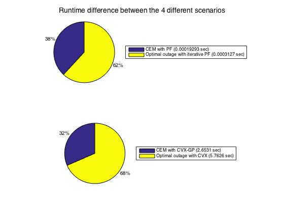
As shown below, the differences between the optimal values of the GP-based CVX and the PF method implementations for both problems are almost zero. This is expected since both methods yeild the optimal answer with very large accuracy.
However, interestingly, there is a significant difference in the runtime of both approaches. Since the experiments vary slightly with respect to time , we have repeated it 5 times and averaged the runtimes for the 4 different approaches. As shown below, The GP-based CVX formulation requires much more time for convergence since it employs the interior point method. The CVX approach for P2 and P1 takes about 2 and 6 seconds, whereas the PF and the iterative PF approaches for P2 and P1 takes about  and
and  seconds, respectively.
disp('Below are additional interesting observations:');
%Additional Analysis (comparison between CVX and PF).
disp([ 'The worst-case optimal CEM_i difference based on PF- and CVX- methods = '...
    num2str(max(abs(1./CEM - CEM_gp))) ]) ;
disp([ 'The worst-case optimal O_i difference based on PF- and CVX- methods = '...
    num2str(max(abs(OOpt_gp - OOpt))) ]) ;
%Additional Timing Analysis.
disp('');
disp([ 'Maximizing Certainty-equivalent margin with PF method = ' ...
    num2str(CEM_toc) ' sec' ]);
disp([ 'Maximizing Certainty-equivalent margin with CVX method = ' ...
    num2str(CEM_gp_toc) ' sec' ]);
disp([ 'Maximizing Certainty-equivalent margin with iterative PF method = ' ...
    num2str(OOpt_toc) ' sec' ]);
disp([ 'Maximizing Certainty-equivalent margin with CVX method = ' ...
    num2str(OOpt_gp_toc) ' sec' ]);
labels = {['CEM with PF (' num2str(CEM_toc) ' sec)' ],['CEM with CVX-GP (' num2str(CEM_gp_toc) ' sec)' ],...
    ['Optimal outage with iterative PF (' num2str(OOpt_toc) ' sec)' ],...
    ['Optimal outage with CVX (' num2str(OOpt_gp_toc) ' sec)' ]};
figure;
suptitle('Runtime difference between the 4 different scenarios');
subplot(2,1,1),
pie([CEM_toc,OOpt_toc]./max([CEM_toc,OOpt_toc]));
legend(labels([1,3]),'Location','eastoutside','Orientation','vertical')
subplot(2,1,2),
pie([CEM_gp_toc,OOpt_gp_toc]./max([CEM_gp_toc,OOpt_gp_toc]));
legend(labels([2,4]),'Location','eastoutside','Orientation','vertical')
Below are additional interesting observations:
The worst-case optimal CEM_i difference based on PF- and CVX- methods = 2.3616e-10
The worst-case optimal O_i difference based on PF- and CVX- methods = 1.5462e-08
Maximizing Certainty-equivalent margin with PF method = 0.00019293 sec
Maximizing Certainty-equivalent margin with CVX method = 2.6531 sec
Maximizing Certainty-equivalent margin with iterative PF method = 0.0003127 sec
Maximizing Certainty-equivalent margin with CVX method = 5.7626 sec
V: Concluding Remarks
In this report, we have reproduced the results of the assigned paper. This project has been very a fruitful experience as we have learnt new concepts in geometric programming such as monomials, psynomials, etc. For the CVX implementations, it was interesting to see that one has to abide by the disciplined convex programming ruleset. For instance, writing the P2(2) constraint as is would not work in CVX since equality is only reserved to "affine=affine". Therefore, the constraint has to be relaxed to ">=" since the left side, namely  is log-concave.
Another interesting observation is that one can express the same problem in many ways with fine differences. We have learnt that employing a heuristic approach based on observations from the problem or the objective function could render a much faster and very accurate approach as compared to simply employing a generic optimization approach such as the interior point method in this scenario.
VI: References
[1] S. Kandukuri and S. Boyd, 'Optimal power control in interference limited fading wireless channels with outage probability specifications,' IEEE Trans. Wireless Commun., vol. 1, no. 1, pp. 46?55, Jan. 2002.
[2] Prakash Chanchana, "An Algorithm For Computing The Perron Root of a Nonnegative Irreducable Matrix" Ph.D. Dissertation, North Carolina State University, Raleigh, 2007 , page 27.
Appendix I: Code of Perron-Frobenius Function
Based on [2], this function implements an effecient algorithm to find PF eigenvector. We note that this has not been used in the report, as we found that it produces similar results to our simple method, given the diagonal regularity of the matrices in our experiments.
function varargout = perron(varargin)
% Function perron(A) computes the perron root of the given square,
% non-negative irreducible matrix.
%
% [r,v] = perron(A, 'right') returns the value of perron root in r and the
% right perron vector in v. Additionally the left perron vector can be
% obtained by passing the string 'left'.
%
% [r,v] = perron(A) returns the perron root and the right perron vector.
%
% [r,v] = perron(A, 'normalized') returns the perron root and perron vector
% of a matrix B = A*inv(D(A)), where D(A) is a diagonal matrix with the
% diagonal entries being the diagonal entries of the matrix A.
%
% [r,v] = perron(A, 'left', 'normalized') returns the perron root and
% perron left vector of a matrix B = A*inv(D(A)), where D(A) is a diagonal
% matric with the diagonal entries being the diagonal entries of the matrix
% A.
%
% Perron root computation is based on the algorithm described in
% PRAKASH CHANCHANA, ``AN ALGORITHM FOR COMPUTING THE PERRON ROOT OF A
% NONNEGATIVE IRREDUCIBLE MATRIX'' Ph.D. Dissertation, North Carolina
% State University, Raleigh, 2007
% Last modified 23-Jan-2009 10:48:43
%

%  Copyright (c) 2009, Aravind Seshadri
%  All rights reserved.
%
%  Redistribution and use in source and binary forms, with or without
%  modification, are permitted provided that the following conditions are
%  met:
%
%     * Redistributions of source code must retain the above copyright
%       notice, this list of conditions and the following disclaimer.
%     * Redistributions in binary form must reproduce the above copyright
%       notice, this list of conditions and the following disclaimer in
%       the documentation and/or other materials provided with the distribution
%
%  THIS SOFTWARE IS PROVIDED BY THE COPYRIGHT HOLDERS AND CONTRIBUTORS "AS IS"
%  AND ANY EXPRESS OR IMPLIED WARRANTIES, INCLUDING, BUT NOT LIMITED TO, THE
%  IMPLIED WARRANTIES OF MERCHANTABILITY AND FITNESS FOR A PARTICULAR PURPOSE
%  ARE DISCLAIMED. IN NO EVENT SHALL THE COPYRIGHT OWNER OR CONTRIBUTORS BE
%  LIABLE FOR ANY DIRECT, INDIRECT, INCIDENTAL, SPECIAL, EXEMPLARY, OR
%  CONSEQUENTIAL DAMAGES (INCLUDING, BUT NOT LIMITED TO, PROCUREMENT OF
%  SUBSTITUTE GOODS OR SERVICES; LOSS OF USE, DATA, OR PROFITS; OR BUSINESS
%  INTERRUPTION) HOWEVER CAUSED AND ON ANY THEORY OF LIABILITY, WHETHER IN
%  CONTRACT, STRICT LIABILITY, OR TORT (INCLUDING NEGLIGENCE OR OTHERWISE)
%  ARISING IN ANY WAY OUT OF THE USE OF THIS SOFTWARE, EVEN IF ADVISED OF THE
%  POSSIBILITY OF SUCH DAMAGE.

normalized = 0;
if nargin < 1
    error('Not enough input arguments')
elseif nargin == 1
    A = varargin{1};
    flag = 'right';
elseif nargin == 2
    A = varargin{1};
    if (strcmp(varargin{2}, 'normalized') || strcmp(varargin{2}, 'Normalized'))
        normalized = 1;
        flag = 'right';
    else
        flag = varargin{2};
    end
elseif nargin == 3
    A = varargin{1};
    flag = varargin{2};
    if (strcmp(varargin{3}, 'normalized') || strcmp(varargin{3}, 'Normalized'))
        normalized = 1;
    else
        error('The third input argument should be the string "normalized"')
    end
else
    error('Too many input arguments')
end

%% Check to see if the input is a square matrix
if ndims(A) > 2
    error('Input to this function should be a n x n square matrix')
else
    [row,column] = size(A);
    if row ~= column
        error('Input to this function should be a n x n square matrix')
    end
end

%% Check if A is non-negative
if max(max(A < 0))
    error('The input matrix should be non-negative')
end

%% Check if A is reducible
% The perron-frobenius theorem is applicable only for nonnegative irreducible matrices
if max(max((A+eye(row))^(row-1) <= 0))
    error('The input matrix is reducible')
end

%% Algorithm to find Perron-Vector

switch flag
    case 'right'
    case 'left'
        A = A.';
end

iterated = rand(row,1);
% Normalize the matrix
if normalized
    A = inv(diag(diag(A)))*A;
end
lambda = max(sum(A));
err = 1;
% This algorithm will fail if A is scalar and of course if A is scalar then
% the perron root is A
if row > 1
    while err > eps
        B = inv(lambda*eye(row) - A);
        [L, U] = lu(lambda*eye(row) - A);
        iterated = L*U\iterated;
        p = iterated./(B*iterated);
        lambda_max = lambda - min(p);
        lambda_min = lambda - max(p);
        err = (lambda_max - lambda_min)/lambda_max;
        iterated = L*U\iterated;
        lambda = lambda_max;
    end
end
perron_root = lambda;
perron_vector = iterated/sum(iterated);

switch nargout
    case 0
        disp(perron_root)
    case 1
        varargout{1} = perron_root;
    case 2
        varargout{1} = perron_root;
        varargout{2} = perron_vector;
    otherwise
        error('Too many output arguments')
end
beep;