Predictive Active Steering Control for Autonomous Vehicle Systems

Connor Fry Sykora - 20620857, Mohammad Sharif Siddiqui - 20342710

1. Problem Formulation
2. Proposed Solution
3. Data Sources
4. Solution
5. Visualization of Results
6. Analysis and Conclusions
6.1 Conclusions
7. Links and References
8. Project Code
8.1 Vehicle Parameters (fitted roughly from source)
8.2 Controller Parameters
8.3 Control Loop
8.4 Error results
9. Plotted Results at current settings (15 m/s)

1. Problem Formulation

Autonomous vehicles calculate the required steering angles required to perform a desired maneuver using automatic controllers. Given some maneuver, Model Predictive Control (MPC) simulates future states of the vehicle based on future steering inputs, then uses optimization techniques to find a set of steering inputs that minimize the deviation of the future states from the desired path, while also minimizing the change in input over the prediction horizon. These predictive controllers are especially useful on low friction roads, where the nonlinear tire behavior dictates the cornering capability of the vehicle.

2. Proposed Solution

In order to determine the optimal steering input, the following optimization in figure 1 is implemented using CVX at each time step:

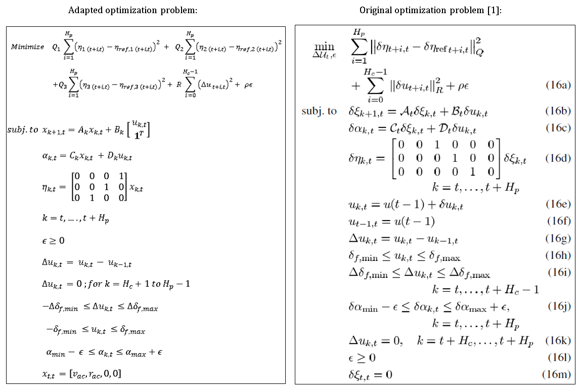
  Figure 1. Controller implemented in project solution compared to original authors' optimization problem.

The adapted implementation (left) is functionally identical to the original algorithm (right). There are slight structural differences that were required since the source publication omits information on the structure of the dynamic model. Justification of these changes is provided in section 4.1. Additionally, since the matrices Q and R are diagonal, the squared quadratic norms present in the objective function can be expressed in CVX as a weighted sum of squared euclidian norms. Explanation of the variables in the optimization scheme are given below in Table I.

The following values are assigned to the parameters to reproduce the results of the linearized model (controller B from the source publication [1])

The implemented code has the order of Q rearranged to match the states (Q1 = 10, Q2 = 200, Q3 = 10). In addition to the above parameters, the controller is also implemented using a control horizon of 1 (controller C from the source publication).

The overall structure of the MPC controller is as follows. Additional details on the steps are found in the 'Solution' section below.

1) Baseline vehicle and controller parameters are established that will be used in the control loop (these parameters are elaborated in the Data Sources section 3.1) Control loop variables are initialized.

2) The control loop is executed over the simulation time, implementing the following steps at each time step:

  a) A prediction of the reference trajectory over the prediction horizon is calculated.
  b) The predicted reference trajectory is translated to the local vehicle coordinate frame (required to maintain linear state matrices)
  c) The current slip angle is used to linearize the state matrices (cornering force is a nonlinear function of slip angle). The linearized matrices are transformed from continuou time to discrete time.
  d) Using CVX, the quadratic objective function is minimized over linear constraint functions.
  e) The first element of the input vector is established as the true steering angle, which is implemented in the linearized dynamic model to simulate the time step.

3) After the completion of the control loop, the maximum and RMS residuals between the true vehicle path and the reference path are calculated.

3. Data Sources

The source publication conducts experiments and simulations for the different controller designs. We will be reproducing the results of the simulations of controllers B and C to the best of our ability given the information available.

3.1 Vehicle Physical Parameters

The source publication provides limited information on the vehicle used in the experiment. The only parameters that are identified are the vehicle mass (2050 kg), the yaw inertia (3344 kg*m^2), and a graph of the nonlinear tire behavior of one wheel as seen in Figure 2 below.

   Figure 2. Lateral tire forces for different road frictions as presented by the source publication.

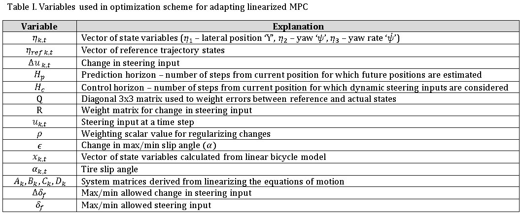
Based solely on this information, the remainder of the vehicle parameters required for implementation were estimated using heuristic knowledge of vehicle dynamics. Using visual inspection of the tire graph and the given inertial properties, the curve fitting constants for the Pacejka magic tire formula were determined [2]. The Pacejka formula was used to determine the cornering capability of the vehicle at each time step. The center of mass location of the vehicle was estimated based on the peak cornering force in the tire model, which corresponds to the normal force on the tire. The estimated parameters are shown below in Table II.

Using these paramters and heuristic knowledge of typical tire behavior, the constants required to use the Pacejka tire model can be derived [2].

3.2 Double Lane Change Trajectory

The authors provide the desired maneuver by defining the global lateral position and the global yaw angle as functions of the global longitudinal position. The equations for the desired maneuver or reference path are given below in Figure 3.

   Figure 3. Equations for generating desired trajectory [1].

Note a typo in the original source [1]; the definitions of yaw and global lateral positions should be reversed. The linearized controller also uses the yaw rate as a trajectory, so the analytical derivative of the yaw angle is calculated for each value of the global lateral position. For the predicted trajectories, it is assumed that the rate of change of the global longitudinal position is constant throughout the prediction, consistent with the methodology of the authors.

3.3 Results Data

Since the majority of the results graphs in the source publication are experimental, only figure 7 from the paper [1] can be used for visual comparison with our simulations. Tabulated results for the simulated controllers B and C are also provided in the source publication, which will be used to quantitatively compare the performance of our controller.

4. Solution

Our script uses CVX to solve a quadratic program with linear constraints. For the internal iterations of the optimization, the stopping criteria and optimization algorithm is determined automatically by CVX. The problem is always feasible, a finite solution is always found. Each optimization requires approximately 0.25s of computation time, meaning that it cannot operate in real-time, which requires a sample time of 0.05s. However, CVX is not optimized for real-time simulations, and the source material indicates that the optimization problem can be solved in less that 0.03s with a suitable solver.

4.1 Changes to Objective and Constraint Functions

As described previously, the adjusted optimization problem preserves the function of the original problem, while employing some structural changes. These changes were necessary due to a lack of information provided by the authors. Specifically, there was no indication of how the state and input matrices were linearized at each time step. Using the single track linear handling model, the original problem formulation does not predict future states and steer inputs, but rather predicts changes in states and steer inputs relative to the current simulated values. Equation 16m in the original formulation indicates that all states are set to zero at the beginning of the prediction horizon (see last constraint in Figure 2). The dynamic model must take into account previous states in order to be physical, which contradicts equation 16m. Subsequently, the previous states are somehow included in the linearization/discretization of the state and input matrices that the authors perform at each time step. Since this technique of linearization is unknown, we have employed an alternate linearization where the matrices are calculated based on the current slip angle (through the Pacejka tire model), and these matrices use the actual states and inputs to predict the behavior. This linearization preserves the physical accuracy of the system.

Equation 16a (objective function in Figure 2) contains a typo that was changed in our implementation (source [1] incorrectly used $\delta$ u instead of $\Delta$ u. This was obviously a typo, since it contradicts the fundamental behavior of MPC and is inconsistent with the nonlinear controller implemented by the authors. The matrix in 16d (see Figure 2) is aesthetically different, indicating the alternative ordering of states in our dynamic model, which is still functionally identical.

The first constraint in Figure 1 which defines the states variables (x_k+1 = A*x_k + B*[u_k; 1]) has a row of ones that are not present in Equation 16b in Figure 2. This is to account for the offset in the linearization of the lateral force curve as shown in Figure 4.

   Figure 4. Linearization of the lateral force curve.

4.2 Localized Reference Trajectories

Before each optimization, translating the reference trajectories from the global coordinates into the local vehicle coordinates is necessary to maintain a linear model. Specifically, the linearized dynamics of the global lateral position ( $\mathit{Y}$ ) results in the product of two states unless the linearization is done about zero yaw angle. Translation of the reference trajectories to the local frame preserves the dynamics, as long as the $\mathit{Y}$ and $\psi$ are set to zero at the beginning of the optimization. The true $\mathit{Y}$ and $\psi$ are calculated using nonlinear dynamics at each time step, after the linear approximation is used in the optimization.

5. Visualization of Results

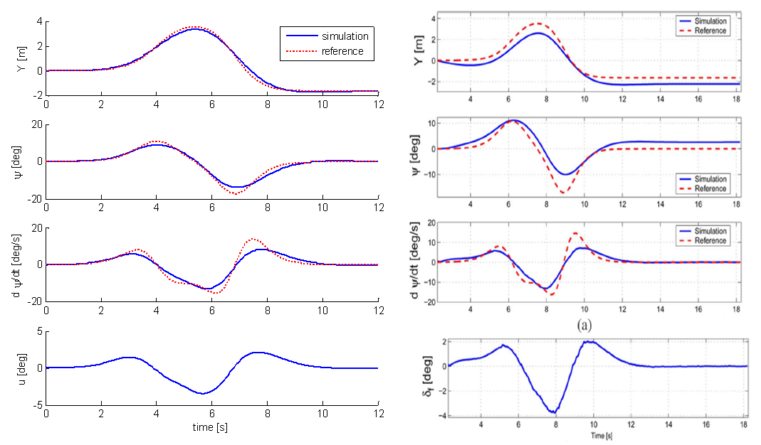
   Figure 5. Reproduced results (left) and published results [1](right) for controller B (Hc = 10) at 10 m/s. Lateral position, Yaw angle, Yaw rate, and steering input.

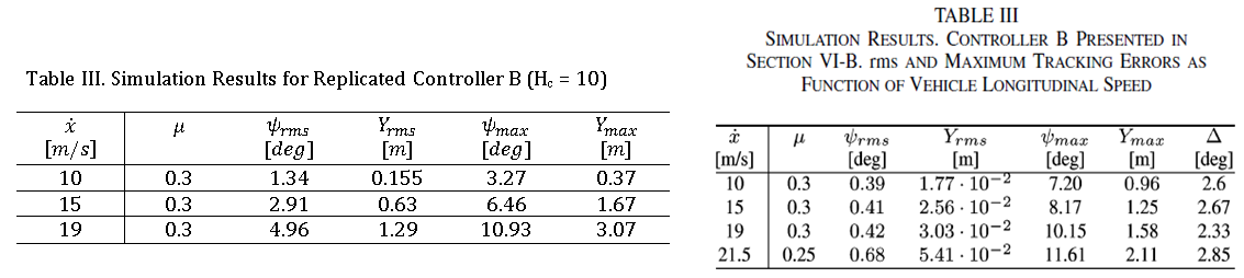
   Figure 6. Reproduced simulation results (left) and published results [1] (right) for controller B (Hc = 10).

   Figure 7. Reproduced simulation results (left) and published results [1] (right) for controller C (Hc = 1).

6. Analysis and Conclusions

As shown in figure 5, our controller implementation matches extremely well with the published results, especially considering the limited vehicle information provided by the authors. Observing the plots for lateral position and yaw angle, the original publication starts its simulation with an heading offset, which is propagated through the simulation and ending with a steady state offset at the end of the maneuver. The authors describe this value ( $\Delta$ in table 3) as an artificial shift of the plot to match with the bias present in their experimental sensors, so this offset in lateral position and yaw is not actually present in their simulation. Therefore, the simulations of the authors match with our results better than the lateral position and yaw plots indicate, which is supported by the comparison of $\mathit{Y}$ max and $\psi$ max.

These maximum values agree well, where our controller performs slightly better at low speeds, but slightly worse at high speeds. The differences can be attributed to three factors:

The differences in vehicle parameters used by the authors versus the values that we had to extract with the limited information provided.
The techniques used to linearize the system matrices. The authors’ technique is unknown, and may be more amenable to the large changes in system behavior over time that are expected at higher speeds.
Given no limits on processing time, CVX was likely able to reach slightly better solutions that the real-time solver used by the original authors.

The RMS error values do not agree well with the published results. This can be easily explained by considering the timescale used to calculate the RMS error. In the published results, the RMS errors were calculated across a fixed time interval, regardless of the test speed. As a result, higher speed maneuvers would end in less time, leaving several error values close to zero at the tails, which artificially lowers the RMS error. Note how the authors’ RMS errors are nearly the same at 10 m/s and 19 m/s, despite a noticeable decrease in maximum error. By contrast, our code automatically detects the start and end of the maneuver based on the reference trajectory, and only uses those values in the calculation of the RMS error. Subsequently, our RMS errors indicate the worse performance of the controller at higher speeds in a similar manner to the maximum errors.

Overall, it is intuitive that errors are higher at higher speeds, since the vehicle will have more difficulty navigating the same maneuver at higher speed, especially on low-friction roads, where higher steering angles saturate the tire lateral force more quickly.

Figure 8 shows a comparison of our simulation of controller B at 19m/s with the original experimental results at 19m/s (The authors do not provide additional simulation plots for controller B, so the experimental results are the only visual point of comparison).

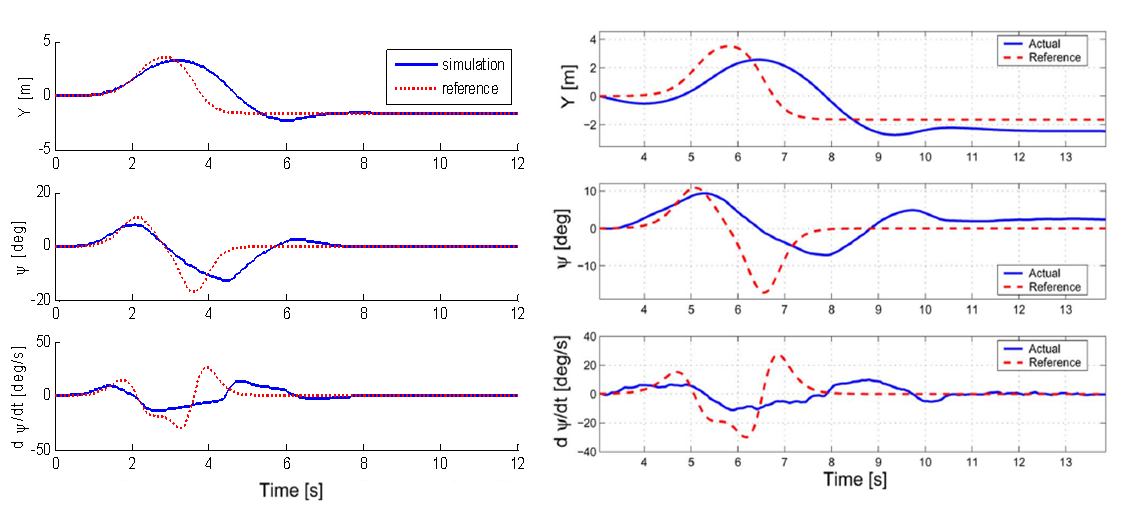
   Figure 8. Simulation results (left) and published experimental results [1] (right) for controller B (Hc = 10) at car speed of 19 m/s.

The plots agree well, although the artificial heading offset is again present in the authors’ plot. This a good indication that our controller produces physically predictable vehicle maneuvers.

The key drawback to this implementation is the choice of prediction horizon given the time step. Predicting 25 timesteps at $\Delta$ t =0.05 is 1.25s. At 19m/s, 1.25s can traverse the harshest part of the maneuver, where the current linearization is far less valid over time. With a lower prediction horizon, the predictions would be more accurate, and the overall computation time would decrease, which is the major limitation of the author’s experiments.

Another notable drawback is that controller C produces better results than controller B. This indicates that the added complexity of controller B degrades from the controller performance. It is possible that setting a constant steer input across the entire prediction is more robust to the linearized dynamics becoming less accurate over time. Controller B may provide better performance over C if the prediction horizon was lower as discussed above.

Another drawback that manifests in physical implementation is the use of global coordinates ( $\mathit{Y}$ and $\psi$ ) in the reference trajectory. Using global variables over vehicle local variables requires an accurate GPS sensor with a high sample rate on the vehicle to locate it in the local frame. Most autonomous vehicle systems plan their trajectories based on LIDAR and object detection, which are measured in the local vehicle reference frame.

6.1 Conclusions

We were able to accurately reproduce the simulation results of the two linearized MPC controllers using CVX. Given limited information on the vehicle configuration and the technique used to linearize the system dynamics, the plots and error values match very well. Despite using a less complicated steering prediction, controller C outperforms controller B, which is consistent with the original publication. Both controllers are able to reasonably navigate a double lane change on a low-friction road at a variety of speeds.

7. Links and References

[1] P. Falcone, F. Borrelli, J. Asgari, H. E. Tseng, and D. Hrovat, "Predictive Active Steering Control for Autonomous Vehicle Systems," IEEE, VOL. 15, NO. 3, MAY 2007

[2] E. Bakker, L. Nyborg, and H. B. Pacejka, "Tyre modeling for use in vehicle dynamics studies," SAE Int., Warrendale, PA, 870421, 1987

Pacejka model used in separate function (Pacejka_F_dF.m)

8. Project Code

8.1 Vehicle Parameters (fitted roughly from source)

m=2050;                 %Vehicle mass (kg) [provided]
J=3344;                 %Vehicle yaw inertia (kg/m^2) [provided]
a=1.045;                %CG to front axle (m)
b=1.453;                %CG to rear axle (m)
dFy_f=70000;            %Front Wheel Cornering Stiffness (N/rad)
dFy_r=55000;            %Rear Wheel Cornering Stiffness (N/rad)
Fn_f=b/(a+b)*2050*9.81; %Front axle normal load (N)
Fn_r=a/(a+b)*2050*9.81; %Rear axle normal load (N)

% CURRENT SETTING FOR VEHICLE SPEED
xdot=15;                %Longitudinal Speed (m/s)


%Pacejka Tire Model
mu=[0.1,0.3,0.5,0.7,0.9];
mu_t=mu(2); %Choose fixed friction for the simulation
%Front Wheel Constants
p_Df=mu_t*Fn_f/2;
peakslip=mu_t*0.17*(70/55);
asym=0.90*p_Df;
p_Cf=1+(1-2/pi*asin(asym/p_Df));
if p_Cf<=1
    p_Cf=1-(1-2/pi*asin(asym/p_Df));
end
p_Bf=dFy_f/(p_Cf*p_Df);
p_Ef=(p_Bf*peakslip-tan(pi/2/p_Cf))/(p_Bf*peakslip-atan(p_Bf*peakslip));
%Rear Wheel Constants
p_Dr=mu_t*Fn_r/2;
peakslip=mu_t*0.17;
asym=0.90*p_Dr;
p_Cr=1+(1-2/pi*asin(asym/p_Dr));
if p_Cr<=1
    p_Cr=1-(1-2/pi*asin(asym/p_Dr));
end
p_Br=dFy_r/(p_Cr*p_Dr);
p_Er=(p_Br*peakslip-tan(pi/2/p_Cr))/(p_Br*peakslip-atan(p_Br*peakslip));

8.2 Controller Parameters

Ts=0.05;         %Sample time
simtime=12;      %Simulation time
t=0:Ts:simtime;  %Global time
Hp=25;           %Prediction Horizon
Hc=10;           %Control Horizon
max_steer=10*pi/180;
max_steerchange=0.85*pi/180;
max_slip=2.2*pi/180;
Q=[10,0,0;0,200,0;0,0,10];
Q1=Q(1,1);
Q2=Q(2,2);
Q3=Q(3,3);
R=50000;
rho=1000;

xi_ac=zeros(4,length(t));   %Actual States
alph_ac=zeros(2,length(t)); %Actual Slip Angles
u_ac=zeros(1,length(t));    %Actual Input
Xac=zeros(1,length(t));     %Actual global lateral position
Xdot_temp=xdot;

eta_ref=zeros(3,Hp,length(t)); %Global Refernce Trajectories
eta_shift=eta_ref;             %Transformed Trajecories (vehicle local frame)
eta_true=zeros(3,length(t));   %Simulated Vehicle Trajectores

dx1=25;                        %Constants that describe the double lane change
dx2=21.95;
dy1=4.05;
dy2=5.7;

%Initialize State Matrices
Ak=zeros(4,4);             %System Matrix
Bk=zeros(4,2);             %Input Matrix
Ck=[-1/xdot,-a/xdot,0,0];  %Output Matrix
Dk=1;                      %Feedforward Matrix
Ak(3:4,:)=[0,Ts,1,0;Ts,0,Ts*xdot,1];

8.3 Control Loop

for i=2:length(t)-1
    %Simulate true reference trajectory based on current X postition
    z1=2.4/25*(Xac(i)-27.19)-1.2;
    z2=2.4/21.95*(Xac(i)-56.46)-1.2;
    eta_true(1,i)=dy1/2*(1+tanh(z1))-dy2/2*(1+tanh(z2)); %Y
    eta_true(2,i)=atan(dy1*(1/cosh(z1))^2*(1.2/dx1)-dy2*(1/cosh(z2))^2*(1.2/dx2)); %psi
    %Generate estimation of reference signal (assume constant X_dot)
    X_cur=Xac(i);  %Current Place on reference curves
    for j=1:Hp
        z1=2.4/25*(X_cur+Xdot_temp*t(j)-27.19)-1.2;
        z2=2.4/21.95*(X_cur+Xdot_temp*t(j)-56.46)-1.2;
        eta_ref(1,j,i)=dy1/2*(1+tanh(z1))-dy2/2*(1+tanh(z2)); %Y_ref
        eta_ref(2,j,i)=atan(dy1*(1/cosh(z1))^2*(1.2/dx1)-dy2*(1/cosh(z2))^2*(1.2/dx2)); %psi_ref
        eta_ref(3,j,i)=-(.2304*dy1*Xdot_temp*sinh(0.96e-1*X_cur+0.96e-1*Xdot_temp*t(j)-3.81024)...
            /(cosh(0.96e-1*X_cur+0.96e-1*Xdot_temp*t(j)-3.81024)^3*dx1)...
            -.2624145785*dy2*Xdot_temp*sinh(.1093394077*X_cur+.1093394077*Xdot_temp*t(j)-7.373302959)/...
            (cosh(.1093394077*X_cur+.1093394077*Xdot_temp*t(j)-7.373302959)^3*dx2))/...
            ((-1.2*dy1/(cosh(0.96e-1*X_cur+0.96e-1*Xdot_temp*t(j)-3.810240000)^2*dx1)...
            +1.2*dy2/(cosh(.1093394077*X_cur+.1093394077*Xdot_temp*t(j)-7.373302959)^2*dx2))^2+1); %r_ref
    end
    %Translate refernce signal to localized coordinates
    for j=1:Hp
        eta_shift(2,j,i)=(eta_ref(2,j,i)-xi_ac(3,i));
        eta_shift(1,j,i)=-Xdot_temp*t(j)*sin(xi_ac(3,i))+...
            (eta_ref(1,j,i)-xi_ac(4,i))*cos(xi_ac(3,i));
        eta_shift(3,j,i)=eta_ref(3,j,i);
    end

    alph_ac(1,i)=atan(Ck*xi_ac(:,i)+Dk*u_ac(i-1));
    alph_ac(2,i)=atan([-1/xdot,b/xdot]*xi_ac(1:2,i));
    [Fc_f,dFy_f]=Pacejka_F_dF(alph_ac(1,i),p_Bf,p_Cf,p_Df,p_Ef); % Current tire force and cornering coefficients
    [Fc_r,dFy_r]=Pacejka_F_dF(alph_ac(2,i),p_Br,p_Cr,p_Dr,p_Er);
    F0_f = Fc_f - dFy_f*alph_ac(1,i);
    F0_r = Fc_r - dFy_r*alph_ac(2,i);
    %Implement Single Track Linear Handling Dynamic Model
    bike_sys=[-2*(dFy_f+dFy_r)/(m*xdot),-2*(dFy_f*a-dFy_r*b)/(m*xdot)-xdot;...
        -2*(dFy_f*a-dFy_r*b)/(J*xdot),-2*(dFy_f*a^2+dFy_r*b^2)/(J*xdot)];
    bike_in=2*[dFy_f/m,(F0_f+F0_r)/m;(dFy_f*a)/J,(F0_f*a-F0_r*b)/J];
    bike_out=[1,0;0,1];
    bike_ff=0;
    %Convert from continuous time to discrete time
    sys=ss(bike_sys,bike_in,bike_out,bike_ff);
    sysd=c2d(sys,Ts);
    [bike_sysd,bike_ind,bike_outd,bike_ffd]=ssdata(sysd);
    Ak(1:2,1:2)=bike_sysd;
    Bk(1:2,1:2)=bike_ind;

    %Perform Optimization over horizon
    cvx_begin quiet
    variable eta_h(3,Hp)
    variable u_h(1,Hp)
    variable delu(1,Hp-1)
    variable xi_h(4,Hp)
    variable alph_h(1,Hp)
    variable epsilon(1)
    minimize(Q1*sum_square(eta_h(1,:)-eta_shift(1,:,i)) ...
        +Q2*sum_square(eta_h(2,:)-eta_shift(2,:,i)) ...
        +Q3*sum_square(eta_h(3,:)-eta_shift(3,:,i)) ...
        +R*sum_square(delu(1:Hc))+rho*epsilon )
    subject to
        xi_h(:,2:Hp)==Ak*xi_h(:,1:Hp-1)+Bk*[u_h(1:Hp-1);ones(1,Hp-1)];
        xi_h(:,1)==[xi_ac(1,i);xi_ac(2,i);0;0]
        alph_h==Ck*xi_h+Dk*u_h
        eta_h==[0,0,0,1;0,0,1,0;0,1,0,0]*xi_h
        epsilon>=0
        delu(1:Hp-1)==u_h(2:Hp)-u_h(1:Hp-1)
        delu(Hc+1:Hp-1)==0
        -max_steerchange<=u_h(1)-u_ac(i-1)<=max_steerchange
        -ones*max_steer<=u_h<=ones*max_steer
        -ones*max_steerchange<=delu<=ones*max_steerchange
        -ones*(max_slip+epsilon)<=alph_h<=ones*(max_slip+epsilon)
    cvx_end
    %Set Steer input for next time step based on optimal prediction
    u_ac(i)=u_h(1);

    %Simulate Time Step
    xi_ac(1:3,i+1)=Ak(1:3,1:3)*xi_ac(1:3,i)+Bk(1:3,:)*[u_ac(i);1];
    xi_ac(4,i+1)=xi_ac(4,i)+Ts*(xdot*sin(xi_ac(3,i))+xi_ac(1,i)*cos(xi_ac(3,i)));
    Xdot_temp=xdot*cos(xi_ac(3,i))-xi_ac(1,i)*sin(xi_ac(3,i));
    Xac(i+1)=Xac(i)+Ts*(Xdot_temp);
end

%Simulate Final Trajectory Step
z1=2.4/25*(Xac(end)-27.19)-1.2;
z2=2.4/21.95*(Xac(end)-56.46)-1.2;
eta_true(1,end)=dy1/2*(1+tanh(z1))-dy2/2*(1+tanh(z2));
eta_true(2,end)=atan(dy1*(1/cosh(z1))^2*(1.2/dx1)-dy2*(1/cosh(z2))^2*(1.2/dx2));

%Numerical differentiation of yaw angle
for i=2:length(t)-1
    eta_true(3,i)=(eta_true(2,i+1)-eta_true(2,i-1))/(2*Ts);
end

8.4 Error results

%Calculate residuals
res=[xi_ac(4,:)-eta_true(1,:);xi_ac(3,:)-eta_true(2,:);xi_ac(2,:)-eta_true(3,:)];

%Truncate Tails for meaningful RMS calculation (only during reference maneuver)
count=0;
for i=1:length(t)
    if abs(eta_true(2,i))>0.003 || abs(eta_true(3,i))>0.003
        trunc_end=i;
        count=count+1;
    end
end
trunc_start=trunc_end-count+1;
res_trunc=res(:,trunc_start:trunc_end);

[max_y,Iy] = max(abs(res_trunc(1,:)));
rms_y = sqrt(mean(res_trunc(1,:).^2));

max_psi = max(abs(res_trunc(2,:)*180/pi));
rms_psi = sqrt(mean(res_trunc(2,:).^2))*180/pi;

9. Plotted Results at current settings (15 m/s)

figure
subplot(4,1,1)
hold on
plot(t,xi_ac(4,:),'LineWidth',2)
plot(t,eta_true(1,:),':','color','r','LineWidth',2)
legend('simulation','reference')
ylabel('Y [m]')
hold off
subplot(4,1,2)
hold on
plot(t,xi_ac(3,:)*180/pi,'LineWidth',2)
plot(t,eta_true(2,:)*180/pi,':','color','r','LineWidth',2)
ylabel('\psi [deg]')
hold off
subplot(4,1,3)
hold on
plot(t,xi_ac(2,:)*180/pi,'LineWidth',2)
plot(t,eta_true(3,:)*180/pi,':','color','r','LineWidth',2)
ylabel('d \psi/dt [deg/s]')
hold off
subplot(4,1,4)
hold on
plot(t,u_ac*180/pi,'LineWidth',2)
ylabel('u [deg]')
xlabel('time [s]')
hold off

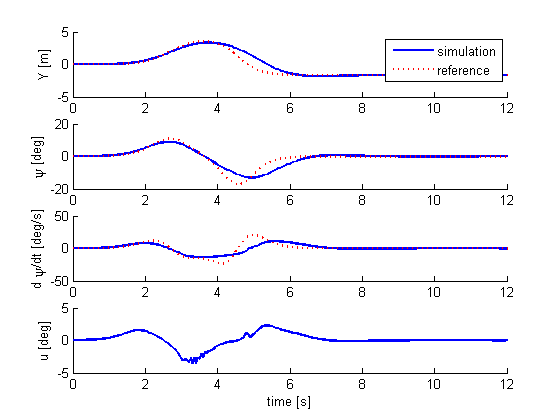
   Figure 9. Simuation resuls for current setting (car speed = 15m/s) using controller B (Hc = 10).