Contents
Learning Inverse Kinematic
%{
Ref:    [1] "Learning inverse Kinematics, Aaron D'Souzam Sethu Vijayakunmar and Stefen Schaal"
        [2] "inverse kinematics,https://en.wikipedia.org/wiki/Inverse_kinematics"
        [3] " Stefan Schaal link:  http://www-clmc.usc.edu/software/lwpr/"
Terminology:
        DOF : Degree of Freedom - The number of free variables in the model

By definition provided in [2], inverse kinematics refers to
the use of the kinematics equation of a robot to determine
the joint parameters that provide a desired position of the end-
effector[2]. The researchers have used a powerful learning
algorithm as a supervised learning algorithm for learning
inverse kinematics. Learning Inverse Kinematic is defined as
real-time control of end-effector which in case of the paper is
for resolved motion rate control (RMRC). Their experiment
is based on augmenting the input space dimension which
is compared to analytical pseudo-inverse with optimization.
Inverse Kinematics problem as mentioned in the paper is the
transformation from kinematics plans in external coordinates to
internal coordinates. Which this inverse transformation results
in ill-posed[1]. As in forward kinematics, the joint coordinates
are in n-dimensional vector of joint angle and the end-effector
as m-dimensional vector. The equation is: x = f(?) where
instead of this forward kinematic function the ? = f?1(x)
which we need to find a optimal solution for later equation
among all possible solutions. In [1] they have proposed a
convex function g = g(?) as criterion so it has global optimum
answer. Finding ? could be solved by 2 approaches as global
approach which is computationally expensive versus local
methods. Local approach is feasible in real time running as
declared in [1] by calculation on ? using x and integrating
? generates entire joint space path [1]. RMRC is this local
approach to the problem. The change of x is described by
Jacobian (J) of the forward Kinematics. x ? = J(?)? ?. In their
project, they have neglected 4 Degree of Freedom (DOF) of
eye and just considered 26 DOF for the humanoid reaching
an object. One solution to minimize g is the a pseudo-inverse
solution: ?? = J#x ? ? ?(I ? J#J) where the general form is:
?? = J^(?1)_E x ?aug.  [1]
------------------------------------------------------------
LWPR Algorithm:
Learning Inverse Kinematics has 2 main advantages. One in case when the
computational complexity of analytical solutions becomes high and second is,
it will not produce ill-conditioned matrix inversion and impossible posture
for humanoid[1]. The major problem is mapping x ? to ? ? which is not a convex
function, however, lots of solutions have been experimented.
Spatially localized learning algorithm is a proper solution.
One supervised method Locally Weighted Projection Regression (LWPR) is a
supervised learining algorithm which takes advantage of piecewise linear
models and each region of validity, receptive field, is derived from a
Gaussian function as:
w_k = exp(?1/2(x ? c_k)T D_k(x ? c_k)) (1)

c_k is center of kth linear model, and D_k is the distance metric that
determines the shape ad size of the regoin of validity of the linear model[1].
The input is x and the output is y k which is weighted mean of all linear
models by equation (2) from [1]:
yHat= (?k=1:K ?kyk)/(?k=1:K ?k) (2)
In LWPR it reformulates the learning function and each step is updated
similar to Newton method.
This code is based on a library, lwpr.m, and test code from following link:
http://www-clmc.usc.edu/software/lwpr/. specially for learning phase of the
process.
---------------------------------------------------------------

%}

function [s,R] = test_lwpr_nD_RmodelIterOpti(s,R)
  global lwprs;

  % Setting up the variables
  d = 5; % input space mapping
  n = 500; % number of samples for LWPR
  inD = 3; % Dimensions of the input
  outD = 2; % Dimensions of the output

  % Random training set using the non-linear function from R3-->R2
  X = (rand(n,inD))*2*pi; % Generation of input space
  Y = [cos(X(:,1)).*sin(X(:,2)), sin(X(:,1)).*cos(X(:,3))];  % Generation of output space
  YnoNoise = Y; % Added noise for storing original function
  Y = Y + randn(n,outD)*0.01; %  Added noise to simulate sensor noise function output
  Yorg = Y;
  disp('data generated');

  % rotate input data into d-dimensional space
  R = randn(d); % Create random set of numbers
  R = R'*R; %  Make it square matrix
  R = orth(R); % make it orthogonal basis as it needed for LWPR library

  Xorg = X;
  X = [X zeros(n,d-3)]*R; % Rotate the input to the new space
  disp('Creating test data');

  % a systematic test set on a grid
  Xt = []; % setting up the trajectory data
  for i=0:0.05:2*pi,
    Xt = [Xt; i pi/4 pi/4];
  end

  Yt = [cos(Xt(:,1)).*sin(Xt(:,2)), sin(Xt(:,1)).*cos(Xt(:,3))]; % setting up the testing dataset

  % rotate the test data according to R matrix
  Xtorg = Xt;
  Xt = [Xt zeros(length(Xt),d-3)]*R;

  % initialize LWPR, use only diagonal distance metric
  ID = 1; % LWPR param
  if ~exist('s') | isempty(s)
    lwpr('Init',ID,d,2,1,0,0,1e-7,50,ones(d,1),[1],'lwpr_test');
  else
    lwpr('Init',ID,s);
  end

  % set some initial parameters setting for the LWPR algorithm from the original
  % sample code
  kernel = 'Gaussian';
  lwpr('Change',ID,'init_D',eye(d)*25);
  lwpr('Change',ID,'init_alpha',ones(d)*100);
  lwpr('Change',ID,'w_gen',0.2);
  lwpr('Change',ID,'meta',1);
  lwpr('Change',ID,'meta_rate',100);
  lwpr('Change',ID,'init_lambda',0.995);
  lwpr('Change',ID,'final_lambda',0.9999);
  lwpr('Change',ID,'tau_lambda',0.9999);
  disp('Training the model');

  % train the model
  for j=1:20
    inds = randperm(n); % Start from random Testing indees
    mse = 0; % re-setting mse variable
    for i=1:n,
      [yp,w,np] = lwpr('Update',ID,X(inds(i),:)',Y(inds(i),:)'); % LWPR for each training point using Update param
      mse = mse + (Y(inds(i),:)'-yp).^2; % calculate mean square error
    end
    nMSE = mse/n/var(Y,1)';	% calculate mse of our data set
    disp(sprintf('#Data=%d #rfs=%d nMSE=%5.3f #proj=%4.2f (TrainingSet)',lwprs(ID).n_data,length(lwprs(ID).rfs),nMSE,np));
  end

  disp('Predicting information');
  % create predictions for the test data (predicted function to show what the model is)
  Yp = zeros(size(Yt)); % initialize output dataset
  for i=1:length(Xt),
    [yp,w]=lwpr('Predict',ID,Xt(i,:)',0.001); % use LWPR for prediction
    Yp(i,:) = yp; % append to output set
  end
  ep   = Yt-Yp; % Difference between actual function and predicted funciton
  mse  = mean(ep.^2); % Mean Square Error
  nmse = mse/var(Y,1);
  disp(sprintf('#Data=%d #rfs=%d nMSE=%5.3f #proj=%4.2f (TestSet)',lwprs(ID).n_data,length(lwprs(ID).rfs),nmse,np));

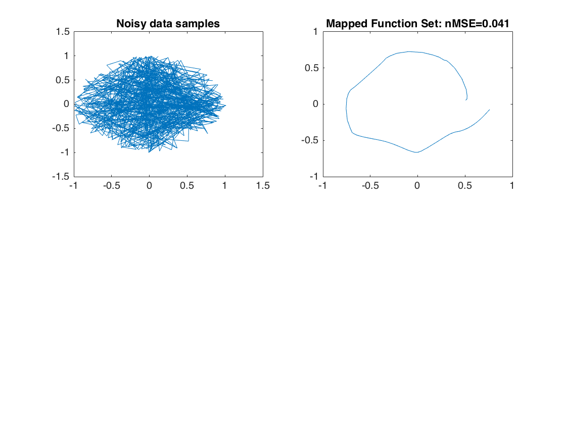
  figure(1);
  clf;

  % plot the raw noisy data
  subplot(2,2,1);
  axis([-1 1 -1 1]);
  plot(Yorg(:,1),Yorg(:,2),'-');
  title('Noisy data samples');

  % plot the fitted function
  subplot(2,2,2);
  axis([-1 1 -1 1]);
  plot(Yp(:,1),Yp(:,2),'-');
  title(sprintf('Mapped Function Set: nMSE=%5.3f',nmse));
data generated
Creating test data
Training the model
#Data=500 #rfs=419 nMSE=0.000 #proj=0.00 (TrainingSet)#Data=9.422855e-01 #rfs=1.004568e+00 nMSE=2.000 #proj=
#Data=1000 #rfs=419 nMSE=0.000 #proj=0.00 (TrainingSet)#Data=8.446115e-01 #rfs=9.220652e-01 nMSE=2.000 #proj=
#Data=1500 #rfs=419 nMSE=0.000 #proj=0.00 (TrainingSet)#Data=4.858839e-01 #rfs=4.926104e-01 nMSE=2.000 #proj=
#Data=2000 #rfs=419 nMSE=0.000 #proj=0.00 (TrainingSet)#Data=2.577122e-01 #rfs=2.454644e-01 nMSE=2.000 #proj=
#Data=2500 #rfs=419 nMSE=0.000 #proj=0.00 (TrainingSet)#Data=1.390693e-01 #rfs=1.480553e-01 nMSE=2.000 #proj=
#Data=3000 #rfs=419 nMSE=0.000 #proj=0.00 (TrainingSet)#Data=1.207992e-01 #rfs=1.339724e-01 nMSE=2.000 #proj=
#Data=3500 #rfs=419 nMSE=0.000 #proj=0.00 (TrainingSet)#Data=6.342840e-02 #rfs=6.727516e-02 nMSE=2.000 #proj=
#Data=4000 #rfs=419 nMSE=0.000 #proj=0.00 (TrainingSet)#Data=4.760527e-02 #rfs=6.315051e-02 nMSE=2.000 #proj=
#Data=4500 #rfs=419 nMSE=0.000 #proj=0.00 (TrainingSet)#Data=4.744065e-02 #rfs=6.298782e-02 nMSE=2.000 #proj=
#Data=5000 #rfs=419 nMSE=0.000 #proj=0.00 (TrainingSet)#Data=4.728728e-02 #rfs=6.284395e-02 nMSE=2.000 #proj=
#Data=5500 #rfs=419 nMSE=0.000 #proj=0.00 (TrainingSet)#Data=4.716327e-02 #rfs=6.271979e-02 nMSE=2.000 #proj=
#Data=6000 #rfs=419 nMSE=0.000 #proj=0.00 (TrainingSet)#Data=4.702750e-02 #rfs=6.259912e-02 nMSE=2.000 #proj=
#Data=6500 #rfs=419 nMSE=0.000 #proj=0.00 (TrainingSet)#Data=2.493273e-03 #rfs=2.253737e-03 nMSE=2.000 #proj=
#Data=7000 #rfs=419 nMSE=0.000 #proj=0.00 (TrainingSet)#Data=2.384653e-03 #rfs=2.149709e-03 nMSE=2.000 #proj=
#Data=7500 #rfs=420 nMSE=0.000 #proj=0.00 (TrainingSet)#Data=2.289735e-03 #rfs=2.054802e-03 nMSE=2.000 #proj=
#Data=8000 #rfs=420 nMSE=0.000 #proj=0.00 (TrainingSet)#Data=2.195507e-03 #rfs=1.970137e-03 nMSE=2.000 #proj=
#Data=8500 #rfs=420 nMSE=0.000 #proj=0.00 (TrainingSet)#Data=2.104682e-03 #rfs=1.891604e-03 nMSE=2.000 #proj=
#Data=9000 #rfs=420 nMSE=0.000 #proj=0.00 (TrainingSet)#Data=2.033538e-03 #rfs=1.821009e-03 nMSE=2.000 #proj=
#Data=9500 #rfs=420 nMSE=0.000 #proj=0.00 (TrainingSet)#Data=1.957919e-03 #rfs=1.747626e-03 nMSE=2.000 #proj=
#Data=10000 #rfs=420 nMSE=0.000 #proj=0.00 (TrainingSet)#Data=1.891221e-03 #rfs=1.681543e-03 nMSE=2.000 #proj=
Predicting information
#Data=10000 #rfs=420 nMSE=0.041 #proj=2.00 (TestSet)

Optimization
%{
   In order to minimize the cost function, as in equation (4), which minimizes
 the distance between optimal theta and given theta gives the
particular solution from [1]. In (4) the given weight determines the
contribution of each DOF in cost function (4).
%
% $$\begin{equation}
    Q = \frac{1}{2} (\dot{\theta}-\hat{\dot{\theta}})^T(\dot{\theta}-\hat{\dot{\theta}}) +\\
        \frac{1}{2}\alpha(\hat{\dot{\theta}}-\frac{\Delta\theta}{\Delta t})^T W(\hat{\dot{\theta}}-\frac{\Delta\theta}{\Delta t})
    \end{equation}
  $$ (4)
%
where in (4) ?? = ?_opt ? ? and W is diagonal weight
matrix where ? is the current prediction given input $z=(x ?,?) $ [1]
cost function is minimized by using equation (5):
% $$\begin{equation}
    \dot{\theta}_{target} = \dot{\theta} - \alpha W (\hat{\dot{\theta}} - \Delta\theta)
    \end{equation}
  $$ (5)
%
  %}
Doing the single-input learning with optimization method
Now plotting additional points Update the model by adding additional data points.
  samples = 500; %number of samples of points
  alpha = 0.6; %The alpha from (12)
  Ypi = zeros(samples,2);

  for i = 1:samples
      idealXi = [i/samples*8*pi pi/4 pi/4]; %set up the optimized case
      Xi = [i/samples*2*pi pi/4 pi/4]; %setup learning data for single point
      Yi = [cos(Xi(1)).*sin(Xi(2)), sin(Xi(1)).*cos(Xi(3))];

      Xaug = Xi  + transpose(alpha.*eye(3)*(Xi - idealXi)'); %Augment point with optimization method
      Xaug = [Xaug zeros(1, d-3)]*R; %rotate input data to d-dimensional space
      [yp,w,np] = lwpr('Update',ID,Xaug(:),Yi(:)); %Update LWPR
      Ypi(i,:) = yp; %Append to output set
  end

  %Plot the data
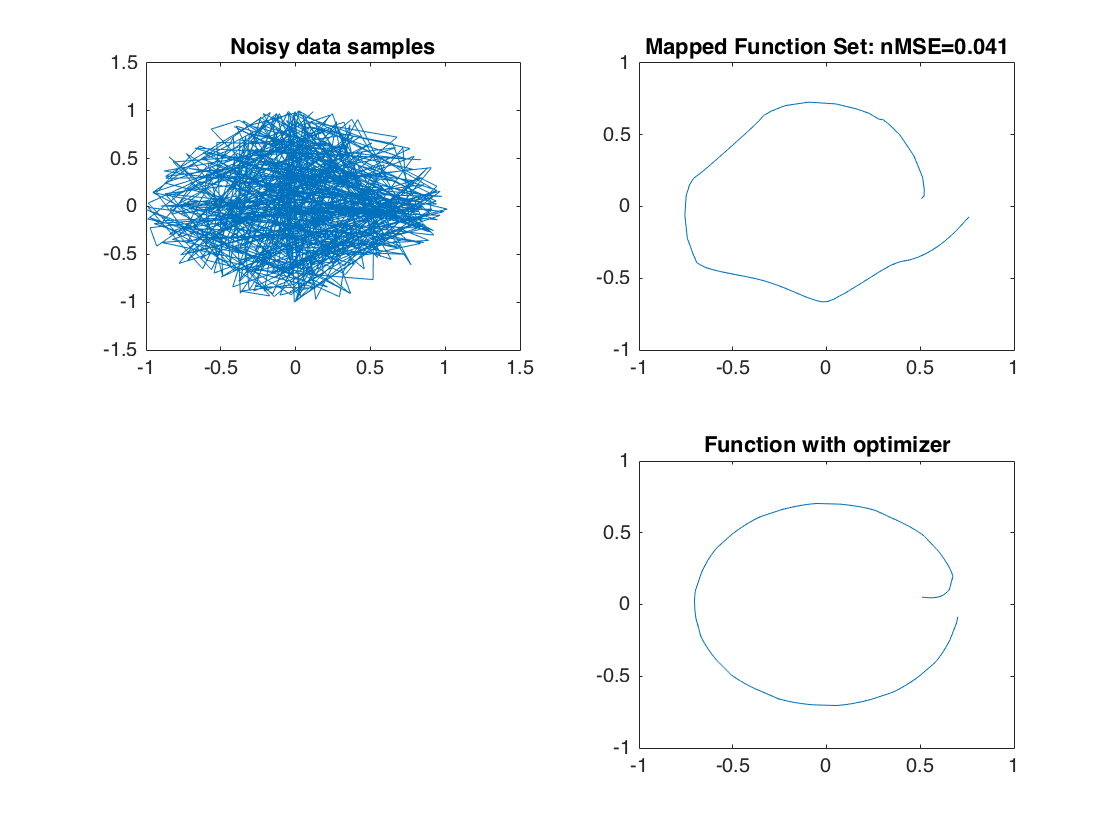
  subplot(2,2,4);
  axis([-1 1 -1 1]);
  plot(Ypi(:,1),Ypi(:,2),'-');
  title('Function with optimizer');

Doing single input learning without the optimization method
  Ypi = zeros(samples,2);
  for i = 1:samples
      Xi = [i/samples*2*pi pi/4 pi/4]; %Mapping trajectory to teach
      Yi = [cos(Xi(1)).*sin(Xi(2)), sin(Xi(1)).*cos(Xi(3))];
      % rotate input data into d-dimensional space
      Xi = [Xi zeros(1,d-3)]*R;
      [yp,w,np] = lwpr('Update',ID,Xi(:),Yi(:));
      Ypi(i,:) = yp;
  end

  %Plot the information.
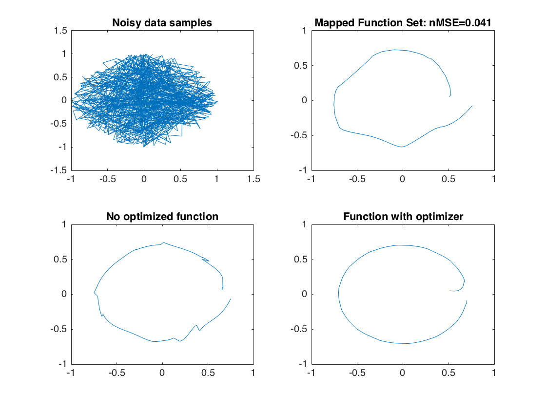
  subplot(2,2,3);
  axis([-1 1 -1 1]);
  plot(Ypi(:,1),Ypi(:,2),'-');
  title('No optimized function');

Conclusion
%{
As the conclusion of the project, by using batch training the results
are not close to optimal desired figure, which in this project the
desired figure is simple circle. However, using single input learning
results in rough figure better than batch learning. By using
optimization cost function where it is biased toward optimal point
($\theta_{opt}$) the result converges to optimal point more accurately.

The following flow-chart is an example of how two tests are operating as
a comparison of between using optimization and without optimizaation:
%                  ________________
%                 | Batch Learning |
%                 |________________|
%                /           \
%               /             \__________
%       _______/____________________    __\_________________________
%   |->|Trajectory Single Input Gen |  |Trajectory Single Input Gen |<-|
%   |  |____________________________|  |____________________________|  |
%   |           |                              |                       |
%   |   ________|__________________     _______|_________              |
%   |_ |LWPR Single Input Learning |   |Optimzer Function|             |
%      |___________________________|   |_________________|             |
%                                       ________|__________________    |
%                                      |LWPR Single Input Learning |___|
%                                      |___________________________|
%
%}