Contents
ECE 602 - PROJECT: Truss Topology Optimization
By: Qing Ge (Christina) Chen & Ginette Wei Get Tseng
clear all; close all; clc;
Problem Formulation
Truss topology design (TTD) is used to design trusses which have fixed element node coordinates[1]. To optimize the TTD, the truss element cross sectional area is varied to minimize the elastic stored energy. The elastic stored energy of the truss element while it is being deflected is used in this optimization problem since deflection of a truss element is unitless.The shortcoming with TTD is that the nodes of the elements are fixed; more optimal designs could be achieved if the nodes are able to migrate slightly from their original positions.
The purpose of this project is to use alternating convex optimization programming to solve for the truss element cross-sectional area and the locations of the nodes of each truss element given specific loading conditions for an optimal truss topology design.
Proposed Solution
The minimization problem looks for the minimum stored elastic energy in the topology, calculated from deflections of the trusses due to an applied force. Change of variables:
are used to cast the problem as a second-order cone program (SOCP). Where  is the internal force in each truss (variable),
  is the force transformation matrix (found geometrically from structure) [2],
  is the node displacement,
  is the truss cross-sectional areas (variable in first problem only).
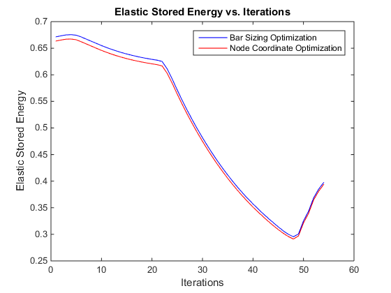
The algorithm is split into two minimization problems with the objective function being the stored elastic energy, then iterated until convergence to obtain the final result. The first problem optimizes truss areas given an initial structure; the second problem optimizes the node locations for the trusses given their areas.
Load Truss Design
The initial truss structure was generated by creating a truss structure similar to the one in [1]. The locations of the nodes are read in from a text file, “node5.txt” and the truss topology is read in from a text file, “elem5.txt”. With format:
![$$[\matrix{node_{num}&x_{position}&y_{positon}}]$$](main_eq11762070646456207145.png)
![$$[\matrix{element_{num}&n_i&n_j}]$$](main_eq14585958187050723737.png)
where  is the
  node and
  is the
  node of the element.
The first and last nodes are fixed nodes that do not migrate; odd and even elements being symmetrical along the y-axis. The number of elements,  , must exceed twice the number of non-fixed nodes
  to ensure that the equality constraint matrix is wide.
% Load node locations from file
    node = load('node5.txt');
    nodenum = node(:,1);                                                        % Node number
    xposn = node(:,2);                                                          % Node x position
    yposn = node(:,3);                                                          % Node y position
    n = length(nodenum);                                                        % Number of nodes

% Load element locations from file
    elem = load('elem5.txt');
    elemnum = elem(:,1);                                                        % Element number
    ni = elem(:,2);                                                             % Element ith node
    nj = elem(:,3);                                                             % Element jth node
    m = length(elemnum);                                                        % Number of elements

% Save initial node positions
    xposn0 = xposn;                                                             % Initial x positions
    yposn0 = yposn;                                                             % Initial y positions
Initialize Parameters for Optimization
Node migration (how much each node would move every iteration) is the same as in [1].  is a vector that stores the first and last nodes so that a boundary condition can be applied. The nodes where the forces are applied are the same as in [1]. Applied forces, Young's modulus the maximum total truss cross-sectional area, and the minimum individual truss cross sectional area were determined arbitrarily. A symmetry constraint was also defined so that migration nodes are symmetrical along the y-axis.
The number of iterations is determined by trial and error.
% Initialize parameters
    E = 70*10^3;                                                                % Young's Modulus(Pa)
    epi = 0.015;                                                                % Node migration rate limit

    fp = [14,1];                                                                % Fixed nodes (descending order)

    N_appx = [];                                                                % Nodes to apply force in x
    N_appy = [3, 6, 8, 10];                                                     % Nodes to apply force in y
    F_appx = 0;                                                                 % Applied force (N) in x
    F_appy = -100;                                                              % Applied force (N) in y

    Amax = 100;                                                                 % Maximum total truss area
    Amin = 1;                                                                   % Minimum individual truss area

    sym = [3,10; 2,13; 4,11; 6,8; 5,12; 7,9];                                   % Rows denote symmetrical nodes of the truss
    iteration = 54;                                                             % Number of interations
Initialize Force Vector
Using initialized external forces and locations, create a force vector for the desired design.
% Initialize force vector
    F = zeros(2*n-2*length(fp), 1);

    for i = 1:length(N_appx)                                                    % Populate applied force vector with values according to initialized parameters
        ind = (N_appx(i)-1)*2-1;
        F(ind) = F_appx;
    end
    for i = 1:length(N_appy)
        ind = (N_appy(i)-1)*2;
        F(ind) = F_appy;
    end
Alternating Convex Optimization Algorithm
CVX is used to set up the two optimization problems. The first optimization problem solves for the truss cross-sectional areas given a fixed topology and applied force. The second problem then uses the cross-sectional areas calculated in the first problem to find how much the nodes can migrate within a given limit to further reduce stored elastic energy, which gives a new fixed topology.
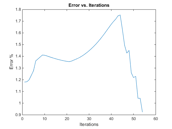
The two problems are iterated until the objective function converges, or by trial and error to find the structure that gives the lowest stored elastic energy. In the presented code, the iteration end condition is set by trial and error.
% Alternating convex optimization algorithm
    for k = 1: iteration

        L = zeros(m,1);                                                     % Initialize truss length vector
        P = zeros(2*n,m);                                                   % Initialize force mapping matrix

        for i = 1:m;
            L(i) = sqrt((xposn(nj(i)) - xposn(ni(i)))^2+...
                (yposn(nj(i)) - yposn(ni(i)))^2);                           % Calculate length of each truss element

            P(2*ni(i)-1, i) = (xposn(nj(i)) - xposn(ni(i)))/L(i);           % Populate force mapping matrix
            P(2*ni(i), i) = (yposn(nj(i)) - yposn(ni(i)))/L(i);
            P(2*nj(i)-1, i) = (xposn(ni(i)) - xposn(nj(i)))/L(i);
            P(2*nj(i), i) = (yposn(ni(i)) - yposn(nj(i)))/L(i);
        end

        for i = 1:length(fp)                                                % Remove rows related to fixed node points
            P(2*fp(i),:) = [];
            P(2*fp(i)-1,:) = [];
        end

        % Bar sizing optimization problem
            cvx_begin quiet
                variables wa(m) va(m) fa(m)
                P*fa + F == 0;
                for i = 1:m;
                    temp(i,:) = [va(i), (L(i)/sqrt(E))*fa(i)];
                    norm(temp(i,:)) <= wa(i);
                end
                wa-va >= Amin;                                              % Area of each truss must exceed the individual minimum area
                ones(1,m)*(wa-va) <= Amax;                                  % Total truss area must not exceed total maximum area
                minimize(ones(1,m)*(wa+va));
            cvx_end

            optim1(k) = ones(1,m)*(wa+va);                                  % Save stored elastic energy for bar size optimization per iteration
            a(:,k) = wa-va;                                                 % Area of truss elements

        % Node coordinate optimization problem
            cvx_begin quiet
                variables wb(m) vb(m) fb(m) yb(2*n-length(fp)*2)
                P*fb + F == 0;
                for i = 1:m;
                    temp2(i,:) = [vb(i), (L(i)/sqrt(E*a(i,k)))*fb(i)];
                    norm(temp2(i,:)) <= wb(i);
                    1/2*((wb(i)-vb(i))-1) == P(:,i)'*yb/L(i);
                end

                for i = 1:(n-length(fp))
                    temp3(i,:) = [yb(2*i-1), yb(2*i)];
                    norm(temp3(i,:)) <= epi;                                % Ensure node migration does not exceed the the predefined value at each iteration
                end
                for i = 1: length(sym(:,1))                                 % Node migration must be symmetrical along y axis
                    xsym1 = (sym(i,1)-1)*2-1;
                    xsym2 = (sym(i,2)-1)*2-1;
                    ysym1 = (sym(i,1)-1)*2;
                    ysym2 = (sym(i,2)-1)*2;

                    yb(xsym1) == -yb(xsym2);
                    yb(ysym1) == yb(ysym2);
                end
                minimize(ones(1,m)*(wb+vb));
            cvx_end

            optim2(k) = ones(1,m)*(wb+vb);                                  % Save stored elastic energy for node coordinate optimization per iteration

        % Calculate new node positions
            bc = [0;0];                                                     % No migration at fixed points
            yb = [bc;yb;bc];                                                % Appended fixed point positions to yb

            delx = yb(1:2:end);                                             % Node migration in x
            dely = yb(2:2:end);                                             % Node migration in y

            xposn = xposn + delx;                                           % New node position in x
            yposn = yposn + dely;                                           % New node position in y

            error(k) = (optim1(k) - optim2(k))/optim2(k);                   % Error in stored elastic energy between two optimization problems

        % Clear temp variables for next iteration
            clearvars temp temp2 temp3
    end
Analysis and Conclusions
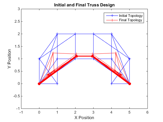
The results in [1] have been reproduced for the most part. We were unable to use the same structure since it required more than 100 iterations in the CVX to solve. A simpler structure is used instead and the results were similar. Since the original problem is non-convex, the convergence may not be the optimal solution. In [1] this was the case and we see the same results in our replication, as seen in the figures.
Some issues with the method is that it is not robust against all loading conditions, if the loadings are not symmetrical and/or are applied at locations on the truss that are not laterally connected to other nodes, the optimization will not be able to find a feasible solution.
% Display results
    figure(1)
    for i = 1:m;                                                            % Plot initial truss topology
        gi = [xposn0(ni(i)) xposn0(nj(i))];
        hi = [yposn0(ni(i)) yposn0(nj(i))];
        plot(gi,hi,'b+-');
        hold on;

        g = [xposn(ni(i)) xposn(nj(i))];
        h = [yposn(ni(i)) yposn(nj(i))];
        w = round(a(i))/5;
        plot(g,h,'r+-', 'LineWidth',w);                                     % Plot final truss topology
        hold on;
    end
    xlabel('X Position');
    ylabel('Y Position');
    title('Initial and Final Truss Design');
    legend('Initial Topology','Final Topology');
    xlim([min(xposn0)-1 max(xposn0)+1]);
    ylim([min(yposn0)-1 max(yposn0)+1]);

    ind = 1:1:k;                                                            % Index for iteration
    figure(2)
    plot(ind, optim1, 'b'); hold on                                         % Plot stored elastic energy for area optimization problem
    plot(ind, optim2, 'r');                                                 % Plot stored elastic energy for node migration optimization problem
    xlabel('Iterations')
    ylabel('Elastic Stored Energy')
    legend('Bar Sizing Optimization','Node Coordinate Optimization');
    title('Elastic Stored Energy vs. Iterations');

    figure(3)
    plot(ind, error*100);                                                   % Plot error between area and node migration optimization results for each iteration
    xlabel('Iterations')
    ylabel('Error %')
    title('Error vs. Iterations');
References
[1] H.Y. Ong and C. Stansbury, "Improving Solutions to the Truss Topology Design Problem with Alternating Convex Optimization," Stanford University, Stanford, CA, June, 2014.
[2] R.M. Freund, "Truss Design and Convex Optimization," Massachusetts Institute of Technology, Cambridge, MA, April, 2004.