Simultaneous Routing and Resource Allocation in CDMA Wireless Data Networks
                  Introduction to optimization
                           ECE 602
Project to fullfill the requirements
of course completion Student Name: Jamal Husain Busnaina
ID. 20641642Winter 2016
Contents
- Problem Description:
- Problem formulation:
- Proposed solution
- Data sources
- Solution
- Algorithm
- Initialization of Assumptions and Given paramaters
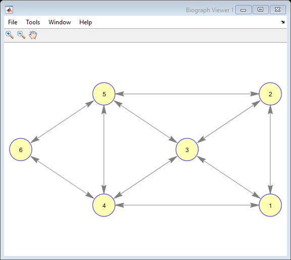
- CDMA network with 6 nodes and 20 directed links - Figure (1)
- Step (a) - Initial network routing and power allocation
- Results of part (a)
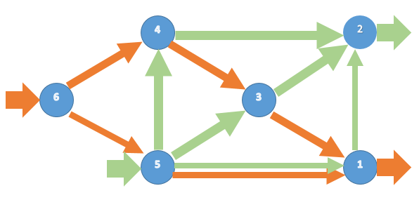
- Initial network routing - Figure 2
- Step (b) - Eliminate Links that have 1 SINR and recalculate optimal routing and power allocation
- Results of part (b)
- Step (c) - Eliminate links that are allocated with very low SINR -"Link 20"
- Results of part (c)
- Final network routing after heuristic procedure - Figure (3)
- Steps and results:
- Analysis and conclusion
Problem Description:
Network routing optimization is task of simultaneous coordination between network’s different layers. The Objective of optimum network performance, can be minimum total power (or bandwidth), minimax power among the nodes, and minimax link utilization. Moreover, to achieve the optimal performance, one must tackle sensitively the task of Optimization problem formulation, which one of its main parts is the constraints imposed by the system nature. One of the main constraints in network routing is Link capacity, which in return, depends on the allocation of transmit power across the network links. Here arise the importance of simultaneous optimization of routing and power allocation in order to obtain optimal performance.
In This paper, a study has been carried out on this joint optimization problem in CDMA data networks using convex optimization techniques.
In CDMA systems, the interference between different links affect the link capacity calculation. Particularly, link capacity depends on the power allocated on the link as well as the power transmitted on other links in the network. Furthermore, the capacity constraints are not jointly convex in communication rates and power allocations. Hence the problem cannot be readily formulated as convex optimization problem. For practical CDMA systems, which are not equipped with interference cancellation, the author suggest coordinate transformation by approximate capacity formula for relatively high signal to interference and noise ratio (SINR) in order to transform the capacity constraint to convex formula.
The project will take into consideration the final formulation of CDMA network without intereference cancellation, and will tackle the numerical problem presented in the paper to demonestrate the results and efficiency of proposed solution to simultaneous routing and resource allocation in CDMA Networks.
Problem formulation:
The network consists of 6 nodes and 20 directed links. The network represented as link-node incidence matrix A. n rows of this matrix indicate the nodes, and l columns indicate the links. A (i,j) = 1 if link j leaves node i , -1 if link j enters node i, or 0 otherwise. In addition to matrix A, B matrix introduced to represent the outgoing links of every node “ -1 elements of A matrix are set to zero”.
Moreover, Number of flow vectors are introduced to formulate this problem, as follow:
1-Source-sink vector Si, for each destination, this vector represent the flow injected in the network at different nodes and destined to sink node i. The nth element indicate the amount of flow supplied by node n that meant to be delivered to node i. where at element n =i shows the total power supplied to node i.
2-flow vector Xi for every destination, the nth element of this vector indicate the amount of flow on link n that is destined to sink node i.
3-Vectors t and c, represent traffic loads and link capacities, respectively.
To represent the interference in CDMA network, the Gain matrix has been considered. The entry Gij is the power gain from the transmitter of link j to the receiver of link i. Intuitively, only diagonal elements of this matrix are desired.
More importantly, the capacity link constraint : after it has been formulated as concave function on variable Q. Where Qi=log(Pi) , Pi : power transmitted at link i. The function:
Capacity of Link i = -log( (noise/Gii) * exp(-Qi) - sum of (i~=j) (Gij/Gii) * exp(Qj - Qi) ) This function is an underestimator of the original formula. Hence, The solution of this function yields feasible solution to the original problem.
The objective is to to maximize the sum throughput of the two flows :
- The flow from source node 6 to sink node 1
- The flow from source node 5 to sink node 2
Proposed solution
Objective Function: maximize(s1+s2)
Variables:
- x1 : flow vector of destination node 1
- x2 : flow vector of destination node 2
- s1 : flow amount inject in the network at node 6, and destined to node 1
- s2 : flow amount inject in the network at node 5, and destined to node 2
- Q : variable of the link capacity function, P=exp(Q)
Formulation of link capacity function.
* k=(G1.*exp(repmat(Q',length(Q),1)-diag(Q)*ones(length(Q),length(Q)))+diag(noise*exp(-Q)))/G2;
* c=-log(sum(k'))
where, c: Link capacity vector, G1 : Gain matrix with diagonal elements set to zero. G2: Diagonal matrix, consists of diagonal elements of Gain matrix|
Constraints:
    Flow conservation constraints
      A*x1==[-s1 0  0 0 0  s1]'     Zero divergences at all nodes except source noed : 6 & 5
      A*x2==[ 0 -s2 0 0 s2  0]'     ans sink nodes : 1& 2
      x1>=0; x2>=0; s2>=0; s1>=0    Flow and divergences of:          - source 6 to sink 1
                                    equal or greater that zero        - source 5 to sink 2
    Link Capacity constraints
     t=x1+x2;                       Traffic load vector
     t<=c'                          Traffic load at every link must be equal or less than its capacity
     B*exp(Q)<=ones(6,1)            sum of transmitted power at every node must be equal or less than 1
The objective function is linear, flow conservation constraints are affine functions. And the link capacity constraints are concave and affine. Therefore, the formulated problem is convex optimization problem. The feasible solution of problem: may have some zero capacity links, which mean that SINR of these links will be 1; because the approximate link capacity function = log(SINR), and zero link capacity enforce SINR to be one. More importantly, these link will be allocated with nonzero power, which show a deficiency in this initial solution. However, The paper propose A heuristic link-removal procedure, which state that these links can be safely removed and gurantee the solution of reduced problem will be feasible. In fact, The performance of the network will be improved, by larger utility or less total power usage.
The procedure which has been taken to solve the problem is as follow: First, using convex optimization solver, find initial solution to the maximum throughput between source and sink nodes. Secondly, investigate the resulting SINR of network links and eliminate link that have SINR with magnitude "one". Repeat these two steps until all SINR of network links are greater that one. Finally, to produce sparser solution, eliminate network links that have very low SINR.
Data sources
Data is generated according to the same numerical example in the paper:
- The network consists of 6 nodes and 20 directed links.
- The noise on the recievers of the links are the same, and equal to 0.001.
- Gain matrix off-diagonal elements are generated randomly with uniform distribution on [0,0.01].
- Gain matrix diagonal elements are equal to one.
- Total Power resource at every node is equal to one.
Solution
Since the problem is formulated as convex optimization problem. And The link capacity constraints are Logarithmic function. This has led us to use cvx toolbox, which has special solver that deal with such sensitive functions.
The approach in this algorithm, for part (b) and (c) was to cancel the effect of the eliminated links in Gain matrix, to free link capacity calculation of the dependency on the power allocated in these links. And discard them as well in the calculation of total power constraints by eliminating their existence in B matrix “matrix of outgoing links”. In addition, capacities of the eliminated links are set to zero. Therefore, the entries in Q variable related to the deleted links are freed and have no effect on the optimal performance of the network.
Stopping criteria :
- Repeat solving the convex optimization problem, eliminate links with zero capacity, until all the SINR of network links are greater than one.
- Eliminate links that have very low SINR, on the expense of slightly less perfomance; but result of sparser routing solution.
In the second step, one must take into account that the solution is not guaranteed to be feasible.
Algorithm
Initialization of Assumptions and Given paramaters
% A matrix :   Incidence matrix represent directed links between nodes
% Node Link  1  2  3  4  5  6  7  8  9 10 11 12 13 14 15 16 17 18 19 20
  r1=      [ 0  0  0  0  0  0 -1  0 -1  1  0  0  0  0  0  0  1  0  1 -1];
  r2=      [ 0  0  0 -1  0  0  0 -1  0 -1  0  0  0  1  0  0  0  1  0  1];
  r3=      [ 0  0  0  0 -1 -1  0  1  1  0  0  0  0  0  1  1  0 -1 -1  0];
  r4=      [-1  0 -1  1  1  0  0  0  0  0  1  0  1 -1 -1  0  0  0  0  0];
  r5=      [ 0 -1  1  0  0  1  1  0  0  0  0  1 -1  0  0 -1 -1  0  0  0];
  r6=      [ 1  1  0  0  0  0  0  0  0  0 -1 -1  0  0  0  0  0  0  0  0];
A=[r1;r2;r3;r4;r5;r6];

% B matrix :   This matrix represent the outgoing links of every node
B=A;
B(B<0)=0;

% Noise    :   Represent the noise at the reciever of a link
              % Here all the recievers have the same noise
noise=0.001;

% Gain matrix: Represent the interefence that is caused by transmitter
              % of link i on receiver of link j

G = 0.01*rand([20 20]);  % Generated Randomly with uniform distribution on [0,0.01]
load('G.mat')            % Previously generated. The work has done based on this set
G=G-diag(diag(G))+diag(ones(20,1));   % Diagonal elements are set to one

G2=diag(diag(G));   % This is diagonal matrix with diagonal elements of Gain matrix
                    % To compact the formula of link capcity function
G1=G-G2;            % This matrix to be used in secon term of capacity link function to compact the formula
                    % Diagonal element are set to zero

% This is to establish the figure of the network to be optimized
C=[0 1 1 1 0 0;1 0 1 0 1 0;1 1 0 1 1 0;1 0 1 0 1 1;0 1 1 1 0 1;0 0 0 1 1 0];
ids = {'1','2','3','4','5','6'};
S=biograph(C,ids,'EdgeType','straight','LayoutScale',0.75,'LayoutType','equilibrium');
CDMA network with 6 nodes and 20 directed links - Figure (1)
view(s)
Step (a) - Initial network routing and power allocation
cvx_begin                                    % Start of convex optimization solver

variables s1(1) s2(1) Q(20) x1(20) x2(20)    % Variables " Data flow are node 6 to 1,  and from node 5 to 2"
                                             % Variables " Q represent Power  P=exp(Q) "
                                             % Variables " xi vector of flow network links destined to node i
maximize(s1+s2)   %Objective Function

%Formulation of link capacity function
k=(G1.*exp(repmat(Q',length(Q),1)-diag(Q)*ones(length(Q),length(Q)))+diag(noise*exp(-Q)))/G2;
c=-log(sum(k'));

%constraints
subject to
     % Flow conservation constraints
     A*x1==[-s1 0  0 0 0  s1]';    % zero diveragences at all nodes expect  source nodes : 6 & 5
     A*x2==[ 0 -s2 0 0 s2  0]';    % and sink nodes : 1 & 2

     x1>=0; x2>=0; s2>=0; s1>=0;   % Flow and divergences of:          - source 6 to sink 1
                                   % equal or greater that zero        - source 5 to sink 2
     % Link Capacity constraints
     t=x1+x2;                      % Traffic load vector
     t<=c'                         % Traffic load at every link must be equal or less than its capacity
     B*exp(Q)<=ones(6,1);          % sum of transmitted power at every node must be equal or less than 1

cvx_end                            % End of optimization problem

% Storing results of step (a)
a_P=exp(Q);
a_SINR=exp(c');
a_x1=x1; a_x2=x2;

% Create Table with results of step (a)
L=[1:20]';
Ta=table(categorical(L),a_SINR,a_P,'VariableNames',{'Link' 'SINR' 'Power_Allocation'});
Ta.Properties.Description = 'Optimal SRRA part (a) = 13.2141';
Successive approximation method to be employed.
   For improved efficiency, SDPT3 is solving the dual problem.
   SDPT3 will be called several times to refine the solution.
   Original size: 1340 variables, 482 equality constraints
   420 exponentials add 3360 variables, 2100 equality constraints
-----------------------------------------------------------------
 Cones  |             Errors              |
Mov/Act | Centering  Exp cone   Poly cone | Status
--------+---------------------------------+---------
404/404 | 8.000e+00  4.886e+00  0.000e+00 | Solved
400/400 | 2.433e+00  3.897e-01  0.000e+00 | Solved
366/366 | 1.776e-01  2.599e-03  0.000e+00 | Solved
204/215 | 6.187e-03  1.767e-06  0.000e+00 | Solved
  0/ 14 | 2.745e-04  3.032e-09  0.000e+00 | Solved
-----------------------------------------------------------------
Status: Solved
Optimal value (cvx_optval): +13.2141
Results of part (a)
Optimal SRRA = 13.2141
disp(Ta)
    Link     SINR     Power_Allocation
    ____    ______    ________________

    1       21.578     0.28806
    2       10.249    0.092025
    3       17.376     0.25188
    4       33.985     0.34391
    5       11.032      0.1261
    6       22.829     0.21505
    7       64.028     0.51741
    8       22.829     0.24286
    9       11.032     0.12195
    10      6.2472    0.092299
    11           1    0.010265
    12           1    0.015664
    13           1    0.016022
    14           1    0.010941
    15           1    0.015096
    16           1     0.01134
    17           1    0.013361
    18           1    0.013403
    19           1    0.010909
    20      1.9559    0.022161
Initial network routing - Figure 2
Step (b) - Eliminate Links that have 1 SINR and recalculate optimal routing and power allocation
%Elimination of unwanted links: The procedure as follow

elim=[11:19];      % Indices of links to be eliminated
A(:,elim)=0;       % Set all the columns representing eliminated links to zero

B=A;               % Calculate reduced matric of outgoing links
B(B<0)=0;

G1(:,elim)=0;       % Set the interefences of eliminated links to zero
G1(elim,:)=0;

% Start of convex optimization solver

cvx_begin
variables s1(1) s2(1) Q(20) x1(20) x2(20)   % Variables " Data flow are node 6 to 1,  and from node 5 to 2"
                                            % Variables " Q represent Power  P=exp(Q) "
                                            % Variables " xi vector of flow network links destined to node i
maximize(s1+s2)  %Objective Function

% Fomulation of link capacity function
k=(G1.*exp(repmat(Q',length(Q),1)-diag(Q)*ones(length(Q),length(Q)))+diag(noise*exp(-Q)))/G2;
c=-log(sum(k'));
c(elim)=0;    % This term is added  to force zero link capacity at eliminated links

% Constraints
subject to
     % Flow conservation constraints
     A*x1==[-s1 0  0 0 0  s1]';    % Zero diveragences at all nodes expect  source nodes : 6 & 5
     A*x2==[ 0 -s2 0 0 s2  0]';    % and sink nodes : 1 & 2

     x1>=0; x2>=0; s2>=0; s1>=0;   % Flow and divergences of:          - source 6 to sink 1
                                   % equal or greater that zero        - source 5 to sink 2
     % Link Capacity constraints
     t=x1+x2;                      % Traffic load vector
     t<=c'                         % Traffic load at every link must be equal or less than its capacity
     B*exp(Q)<=ones(6,1);          % Sum of transmitted power at every node must be equal or less than 1

cvx_end                            % End of optimization problem

% Storing results of step (b)
b_P=exp(Q);
b_SINR=exp(c');
b_x1=x1; b_x2=x2;
b_P(11:19)=0;b_SINR(11:19)=0;
% Create Table with results of step (b)
Tb=table(categorical(L),b_SINR,b_P,'VariableNames',{'Link' 'SINR' 'Power_Allocation' });
Tb.Properties.Description = 'Optimal SRRA part (b) = 13.4348';
Successive approximation method to be employed.
   SDPT3 will be called several times to refine the solution.
   Original size: 907 variables, 307 equality constraints
   130 exponentials add 1040 variables, 650 equality constraints
-----------------------------------------------------------------
 Cones  |             Errors              |
Mov/Act | Centering  Exp cone   Poly cone | Status
--------+---------------------------------+---------
124/124 | 8.000e+00  1.323e+01  0.000e+00 | Solved
124/124 | 7.000e+00  1.897e-01  0.000e+00 | Solved
115/119 | 7.000e+00  5.791e-04  0.000e+00 | Solved
 35/ 65 | 7.000e+00  4.356e-07  0.000e+00 | Solved
  0/  0 | 7.000e+00  0.000e+00  0.000e+00 | Solved
-----------------------------------------------------------------
Status: Solved
Optimal value (cvx_optval): +13.4348
Results of part (b)
Optimal SRRA = 13.4348
disp(Tb)
    Link     SINR     Power_Allocation
    ____    ______    ________________

    1       22.087     0.28152
    2       10.715    0.091089
    3       18.104      0.2515
    4       34.726     0.34215
    5       11.515     0.12658
    6       24.482     0.21614
    7       69.807     0.53236
    8       24.482     0.24462
    9       11.515      0.1195
    10      6.5149    0.092659
    11           0           0
    12           0           0
    13           0           0
    14           0           0
    15           0           0
    16           0           0
    17           0           0
    18           0           0
    19           0           0
    20      1.9181    0.020026
Step (c) - Eliminate links that are allocated with very low SINR -"Link 20"
%Elimination of unwanted links: The procedure as follow

elim=[11:20];      % Indices of links to be eliminated
A(:,elim)=0;       % Set all the columns representing eliminated links to zero

B=A;               % Calculate reduced matric of outgoing links
B(B<0)=0;

G1(:,elim)=0;       % set the interefences of eliminated links to zero
G1(elim,:)=0;


%Start of optimization program
cvx_begin

variables s1(1) s2(1) Q(20) x1(20) x2(20)  % Variables " Data flow are node 6 to 1,  and from node 5 to 2"
                                           % Variables " Q represent Power  P=exp(Q) "
                                           % Variables " xi vector of flow network links destined to node i
maximize(s1+s2)   %Objective Function

%Fomulation of link capacity function
k=(G1.*exp(repmat(Q',length(Q),1)-diag(Q)*ones(length(Q),length(Q)))+diag(noise*exp(-Q)))/G2;
c=-log(sum(k'));
c(elim)=0;   % This term is added to force zero link capacity at eliminated links

%Constraints
subject to
     % Flow conservation constraints
     A*x1==[-s1 0  0 0 0  s1]';    % zero diveragences at all nodes expect  source nodes : 6 & 5
     A*x2==[ 0 -s2 0 0 s2  0]';    % and sink nodes : 1 & 2

     x1>=0; x2>=0; s2>=0; s1>=0;   % Flow and divergences of:          - source 6 to sink 1
                                   % equal or greater that zero        - source 5 to sink 2
     % Link Capacity constraints
     t=x1+x2;                      % Traffic load vector
     t<=c'                         % Traffic load at every link must be equal or less than its capacity
     B*exp(Q)<=ones(6,1);          % sum of transmitted power at every node must be equal or less than 1


cvx_end

% Storing result of step (c)
c_P=exp(Q);
c_SINR=exp(c');
c_x1=x1; c_x2=x2;
c_SINR(11:20)=0;
c_P(11:20)=0;
% Create Table with results of step (c)
Tc=table(categorical(L),c_SINR,c_P,'VariableNames',{'Link' 'SINR' 'Power_Allocation' });
Tc.Properties.Description = 'Optimal SRRA part (c) = 13.3627';
Tt=table(categorical(L),a_SINR,b_SINR,c_SINR,a_P,b_P,c_P,'VariableNames',{'Link' 'a_SINR' 'b_SINR' 'c_SINR' 'a_Power_Allocation' 'b_Power_Allocation' 'c_Power_Allocation'});
Successive approximation method to be employed.
   SDPT3 will be called several times to refine the solution.
   Original size: 844 variables, 265 equality constraints
   109 exponentials add 872 variables, 545 equality constraints
-----------------------------------------------------------------
 Cones  |             Errors              |
Mov/Act | Centering  Exp cone   Poly cone | Status
--------+---------------------------------+---------
103/103 | 8.000e+00  1.383e+01  0.000e+00 | Solved
102/102 | 1.112e+00  7.671e-02  0.000e+00 | Solved
 96/ 99 | 4.551e-02  1.320e-04  0.000e+00 | Solved
  4/ 63 | 6.757e-04  2.624e-08  0.000e+00 | Solved
  0/  0 | 6.165e-05  0.000e+00  0.000e+00 | Solved
-----------------------------------------------------------------
Status: Solved
Optimal value (cvx_optval): +13.3627
Results of part (c)
Optimal SRRA = 13.3627
disp(Tc)
    Link     SINR     Power_Allocation
    ____    ______    ________________

    1       15.403     0.18949
    2       10.215     0.08594
    3       24.438     0.31655
    4       24.438      0.2399
    5       15.403     0.15078
    6       24.527     0.19751
    7       68.871     0.48595
    8       24.527     0.24113
    9       15.403     0.14143
    10       6.742    0.087601
    11           0           0
    12           0           0
    13           0           0
    14           0           0
    15           0           0
    16           0           0
    17           0           0
    18           0           0
    19           0           0
    20           0           0
Final network routing after heuristic procedure - Figure (3)
Steps and results:
- The initial solution at step (a) is shown in figure (2) , the total throughput is 13.2141.
- At step (b), we removed links from 11 to 19 that have SINRs equal to one, the resulting routing pattern is the same, and total throughput has improved to 13.4348.
- Finally at step (c), we removed link 20 that have the lowest SINR , resulting network routing is shown in figure (3), which has sparser network routing than the initial routing solution. However, the total throughput decreased slightly to 13.3627.
disp(Tt)
    Link    a_SINR    b_SINR    c_SINR    a_Power_Allocation    b_Power_Allocation    c_Power_Allocation
    ____    ______    ______    ______    __________________    __________________    __________________

    1       21.578    22.087    15.403     0.28806               0.28152               0.18949
    2       10.249    10.715    10.215    0.092025              0.091089               0.08594
    3       17.376    18.104    24.438     0.25188                0.2515               0.31655
    4       33.985    34.726    24.438     0.34391               0.34215                0.2399
    5       11.032    11.515    15.403      0.1261               0.12658               0.15078
    6       22.829    24.482    24.527     0.21505               0.21614               0.19751
    7       64.028    69.807    68.871     0.51741               0.53236               0.48595
    8       22.829    24.482    24.527     0.24286               0.24462               0.24113
    9       11.032    11.515    15.403     0.12195                0.1195               0.14143
    10      6.2472    6.5149     6.742    0.092299              0.092659              0.087601
    11           1         0         0    0.010265                     0                     0
    12           1         0         0    0.015664                     0                     0
    13           1         0         0    0.016022                     0                     0
    14           1         0         0    0.010941                     0                     0
    15           1         0         0    0.015096                     0                     0
    16           1         0         0     0.01134                     0                     0
    17           1         0         0    0.013361                     0                     0
    18           1         0         0    0.013403                     0                     0
    19           1         0         0    0.010909                     0                     0
    20      1.9559    1.9181         0    0.022161              0.020026                     0
Analysis and conclusion
We have demonstrated the efficiency of simultaneous routing and resource allocation formulation proposed by the paper. The transformation that has been done on the approximated link capacity function, for CDMA network without interference cancellation, produced concave link capacity function. The SRRA problem was formulated readily as convex optimization problem and the optimal performance was obtained efficiently. Moreover, the heuristic procedure improved the performance of the network in terms of throughput, and power utilization.
The results of numerical example has been demonstrated. Although gain matrix was generated randomly, the final routing pattern is the same as the results in the paper.
1- It should be noticed that the approximated formulation of the link capacity, assuming to deal with high SINR CDMA networks. Implementation of this formula on low SINR network may not result in feasible solutions.
2- High SINR network has allowed us to delete links with very low SINR, but feasibility is not guaranteed as stated by the author. Also, this procedure will be much difficult if the SINRs of the network links were low.
3- The approximated formula to link capacity requires the SINR to be equal or larger than one. Moreover, the variable transformed Q= log (P), oblige the optimization solver to allocate all the links with nonzero power. This is what imposed the necessity of heuristic procedure to achieve the optimal performance, so the heuristic approach is mandatory when using this approximated formula. As a result,the algorithm on this project had to approach the link elimination procedure indirectly by manipulating total power allocation constraints, and Gain matrix.
4- Optimal routing performance is operational action in data network, it requires very fast decision making. However, solving the optimization problem multiple times to achieve the optimal routing solution, and the logarithmic nature of link capacity constraints, consume considerable amount of time; and that make the application of this algorithm under the hardware and software of this project is not time effective.
In conclusion, the convex optimization techniques are very powerful tools to solve optimization problems. To solve problem as convex optimization problem, several concerns have to be taken into account:
• Careful investigation of the problem to consider all the aspects of the problem's nature and constraints
• Skills and knowledge to apply coordinate projection and transformation on the problem function in order to obtain convex functions.
• Finally, formulation of the objective and the constraints as convex optimization problem
“With only a bit of exaggeration if you formulate a practical problem as a convex optimization problem, then you have solved the original problem." (S. Boyd)