"Finding Ultimate Limits of Performance for Hybrid Electric Vehicles"[1]
An exercise in recreating the results from Tate and Boyd's Paper
Contents
By Sindhura Buggaveeti and Allison Waters
Problem Description
  In this project, the objective was to reproduce the results from Tate
and Boyd's paper, "Finding ultimatelimits of performance for hybrid
electric vehicles" [1]. The article proses problem of finding optimal
engine operation in a pure series hybrid vehicle over a fixed drive cycle
subject to a number of practical contraints such as nonlinear fuel/power
maps, minimum and maximum battery charge, battery efficiency, nonlinear
vehicle dynamics and losses, drive train efficiency, engine slew rate
limits.
- Nonlinear fuel/power maps
- Min and max battery charge
- Battery efficiency
- Nonlinear vehicle dynamics and losses
- Drive train efficiency
- Engine slew rate limits
The problem of optimizing fuel efficiency is initially formulated as a
nonlinear convex optimization problem. This convex problem is then
accurately approximated as a large linear program. This optimal solution
is the lower limit of fuel consumption that any control law can achieve
for the given drive cycle and vehicle.
Proposed Solution

Objective function for optimal fuel economy can be described as:

Following are the equality and inequality constraints for the proposed optimization problem.


The parameters and variable described in the above algorithm are:
* Variables: $$f(k), E(k), P_e(k), P_b(k), P_s(k)$$
* Parameters: Max Engine Slew Up, Max Engine Slew Down, Max Engine
Power, Max Braking Power, Max Discharge and charge rate, Min and Max
BatteryEnergy
   The optimization problem above was converted into a convex linear
program and solved using Grant and Boyd's convex optimization software
for Matlab, CVX [2][3].
Data Sources
  To illustrate the results obtained using this method, a numerical
example was performed. The drive cycle is first 1371 seconds of FTP-75
Urban Dynamometer Driving Schedule'(UDDS) [4]. The vehicle mass is 1072kg
with a coefficient of drag(CD) of 0.3 and frontal area of 1.96m^2. The
coefficient of rolling resistance is 0.015. Air density is 1.22kg/m^3.
The vehicle is modeled with a 2kW battery load. The fuel consumption
curve for engine is approximated by


where f(t) is in unit of grams per second and P_e is in units of W.
The battery is lead acid(PbA) with 0.60 kW-hr maximum energy capcity and
a reserve of 0.12 KW-hrs. The maximum charge and discharge rates are
9.54kW. The battery has a charge efficiency of 80% and discharge
efficiency of 100% as given in the paper.
Solution for Hybrid Vehicle
Input Parameters
The mechanical power generated by the vehicle is calculated by the
equation below using the following inputs given in the paper.

Vel=xlsread('FTP.xlsx');    %FTP drive cycle data [4]
m=1072;     %Mass of vehicle
Cd=0.3;     %Coefficient of drag
A=1.96;     %Frontal Area
Cr=0.015;   %Rolling resistance coefficient
p=1.22;     %Density of air
g=9.81;     %Gravity
k=1371;     %Number of discrete time steps (each time step is 1 second)
V=0;        %Initial velocity
g1=0.8;     %Battery charge efficiency
g2=1;       %Battery discharge efficiency
ve=0.44704*Vel;  %Converting FTP velocity from mph to m/s
for i=1:k
    %Vehicle acceleration using derivative approximation
    a(i,1)=ve(i)-V;
    %Updating V to be the previous velocity for the next acceleration
    %calculation
    V=ve(i);
    %Calculating mechanical power required to drive the vehicle
    Pm(i,1)=(0.5*p*Cd*A*(ve(i,1)^2)+m*g*(Cr+a(i,1)/g))*ve(i,1)/1000+2;
    time(i)=i;          %Time in seconds
end
Matrices and arrays
one=ones(1,k);              %lxk matrix of ones
none=one(1,1:k-1);         %1xk-1 matrix of ones
%D is an "identity" matrix with -1 along diagonal and 1 along diagonal one
%above the center diagonal
D=-diag(one)+diag(none,1);
Z=zeros(k);                 %kxk matrix of zeros
T=eye(k);                   %kxk identity matrix
Onit=ones(k,1);             %kx1 matrix of ones
ED=D;               %ED is a kxk identity matrix with the element (k,k)=0
ED(k,k)=0;
c=zeros(1,8*k);
c(1,1:k)=one;
Generating equality constraint matrices
The matrix equality constraint Ax==b is made from the equality equations
where A is a (4*k+1)x11*k matrix and b is a (4*k+1)x1 matrix. Slack and surplus
variables were added to 2 equations to convert the inequality
constraints that could cause the set of feasible solutions to degenerate
the rank of the constraints into equality constraints. The storage power
of the battery (Ps) was split into positive (Psp) and negative values
(Psn) so that the variables, Psp and Psn, could be positive. It is
required that all variables in the linear program be greater than zero.
The battery power was determined from the equation below.

By substituting the equation for battery power into the constraints,
Ax==b consisted of the following 5 equations:


A1=[T,-0.059.*T,-T,Z,Z,Z,Z,Z;-T,0.096.*T,Z,T,Z,Z,Z,Z;Z,T,Z,Z,T,-T,-T,Z;Z,Z,Z,Z,T,-0.8.*T,Z,ED];
A=zeros(4*k+1,8*k);
A(4*k+1,7*k+1)=1;
A(4*k+1,8*k)=-1;
A(1:4*k,1:8*k)=A1+A(1:4*k,1:8*k);

b=zeros(4*k+1,1);               %Initializing b
b(1:k,1)=0.075.*Onit;           %Equation 1 right side
b(k+1:2*k,1)=1.041667.*Onit;    %Equation 2 right side
b(2*k+1:3*k,1)=Pm;              %Equation 3 right side
Generating inequality constraint matrices
The matrix inequality constraint Gx<=H was made from the inequality
equations where G is a 7*kx11*k matrix and H is a 7*kx1 matrix. The
inequality constraints consist of the upper bound limits on the four
parameters Pe, Psp, Psn, Pb, E, and the upper bound limits on the rate
of change in engine supply power (Pe). In total, 7 equations were
combined to make the matrix inequality constraint.


G=[Z,T,Z,Z,Z,Z,Z,Z;Z,Z,Z,Z,T,Z,Z,Z;Z,Z,Z,Z,Z,T,Z,Z;Z,Z,Z,Z,Z,Z,T,Z;Z,Z,Z,Z,Z,Z,Z,T;Z,D,Z,Z,Z,Z,Z,Z;Z,-D,Z,Z,Z,Z,Z,Z];
H=[50.*Onit;9.54.*Onit;6.875.*Onit;13.585.*Onit;2160.*Onit;10.*Onit;20.*Onit];
CVX Code
With the additions of slack and surplus variables, the total number of
variables in the convex optimization problem is 10968 with 8 vectors
each with 1371 elements (the vectors are fuel consumption (f), engine
power (Pe), surplus variable (s1), slack variable (s2), negative storage
power (Psn), positive storage power (Psp), brake power (Pb), battery
energy (E)). The problem is a linear program optimization problem,
therefore, all of the variables must be positive. The battery energy has
a minimum value constraint that it must be greater than 432
kiloWatt-seconds.
cvx_begin
    variables x(8*k,1)
    minimize c*x
    subject to
        A*x==b
        G*x<=H
        x>=0
        x(7*k+1:8*k,1)>=432
cvx_end
Calling SDPT3 4.0: 23305 variables, 6853 equality constraints
   For improved efficiency, SDPT3 is solving the dual problem.
------------------------------------------------------------

 num. of constraints = 6853
 dim. of linear var  = 21935
 dim. of free   var  = 1370
 *** convert ublk to linear blk
********************************************************************************************
   SDPT3: homogeneous self-dual path-following algorithms
********************************************************************************************
 version  predcorr  gam  expon
    NT      1      0.000   1
it pstep dstep pinfeas dinfeas  gap     mean(obj)    cputime    kap   tau    theta
--------------------------------------------------------------------------------------------
 0|0.000|0.000|8.7e+03|5.6e+03|2.7e+11| 1.868927e+08| 0:0:00|2.7e+11|1.0e+00|1.0e+00| spchol 1   1
 1|0.000|0.000|8.7e+03|5.6e+03|2.7e+11| 1.868928e+08| 0:0:00|2.7e+11|1.0e+00|1.0e+00| spchol 1   1
 2|0.000|0.000|8.7e+03|5.6e+03|2.7e+11| 1.868930e+08| 0:0:00|2.7e+11|1.0e+00|1.0e+00| spchol 1   1
 3|0.000|0.000|8.7e+03|5.6e+03|2.7e+11| 1.868942e+08| 0:0:00|2.7e+11|1.0e+00|1.0e+00| spchol 1   1
 4|0.000|0.000|8.7e+03|5.6e+03|2.7e+11| 1.868992e+08| 0:0:00|2.7e+11|1.0e+00|1.0e+00| spchol 1   1
 5|0.000|0.000|8.7e+03|5.6e+03|2.7e+11| 1.869138e+08| 0:0:00|2.7e+11|1.0e+00|1.0e+00| spchol 1   1
 6|0.000|0.000|8.7e+03|5.6e+03|2.7e+11| 1.869579e+08| 0:0:00|2.7e+11|1.0e+00|1.0e+00| spchol 1   1
 7|0.001|0.001|8.6e+03|5.6e+03|2.7e+11| 1.870899e+08| 0:0:00|2.6e+11|1.0e+00|1.0e+00| spchol 1   1
 8|0.003|0.003|8.6e+03|5.6e+03|2.6e+11| 1.874855e+08| 0:0:00|2.6e+11|1.0e+00|1.0e+00| spchol 1   1
 9|0.010|0.010|8.6e+03|5.5e+03|2.6e+11| 1.886679e+08| 0:0:00|2.6e+11|1.0e+00|9.9e-01| spchol 1   1
10|0.030|0.030|8.4e+03|5.4e+03|2.6e+11| 1.921746e+08| 0:0:00|2.6e+11|9.9e-01|9.6e-01| spchol 1   1
11|0.088|0.088|7.9e+03|5.1e+03|2.6e+11| 2.023113e+08| 0:0:00|2.4e+11|9.8e-01|8.9e-01| spchol 1   1
12|0.253|0.253|6.5e+03|4.2e+03|2.2e+11| 2.288910e+08| 0:0:00|1.9e+11|9.4e-01|7.0e-01| spchol 1   1
13|0.630|0.630|2.9e+03|1.8e+03|1.1e+11| 2.731481e+08| 0:0:00|7.7e+10|9.0e-01|3.0e-01| spchol 1   1
14|0.966|0.966|1.0e+02|6.8e+01|4.6e+09| 2.682438e+08| 0:0:00|1.4e+09|9.1e-01|1.1e-02| spchol 1   1
15|0.764|0.764|2.3e+01|1.5e+01|8.5e+08| 6.016079e+07| 0:0:00|3.7e+07|1.1e+00|2.9e-03| spchol 1   1
16|0.790|0.790|5.0e+00|3.2e+00|1.6e+08| 1.204795e+07| 0:0:00|1.0e+06|1.3e+00|7.4e-04| spchol 1   1
17|0.808|0.808|1.1e+00|6.2e-01|2.6e+07| 4.318146e+06| 0:0:01|2.5e+04|1.5e+00|1.7e-04| spchol 1   1
18|0.853|0.853|1.0e+00|9.8e-02|3.7e+06| 9.697342e+05| 0:0:01|6.4e+02|1.8e+00|3.1e-05| spchol 1   1
19|0.966|0.966|3.3e-01|5.3e-03|2.1e+05| 5.125682e+04| 0:0:01|2.2e+02|2.0e+00|1.7e-06| spchol 1   1
20|0.960|0.960|1.3e-02|6.6e-04|8.6e+03| 4.064272e+03| 0:0:01|2.3e+01|2.0e+00|7.1e-08| spchol 1   1
21|0.905|0.905|4.1e-03|5.1e-04|4.5e+03| 3.207877e+03| 0:0:01|2.8e+00|2.0e+00|3.2e-08| spchol 1   1
22|1.000|1.000|1.3e-03|4.0e-04|1.5e+03| 2.473243e+03| 0:0:01|3.6e-01|2.0e+00|9.4e-09| spchol 1   1
23|0.966|0.966|5.4e-04|3.5e-04|8.2e+02| 2.331539e+03| 0:0:01|1.3e-01|2.0e+00|5.2e-09| spchol 1   1
24|1.000|1.000|1.3e-04|3.1e-04|1.9e+02| 2.197099e+03| 0:0:01|6.6e-02|2.0e+00|1.2e-09| spchol 1   1
25|0.938|0.938|9.5e-05|2.8e-04|1.1e+02| 2.185700e+03| 0:0:01|1.9e-02|2.0e+00|6.8e-10| spchol 1   1
26|1.000|1.000|2.7e-05|2.5e-04|2.7e+01| 2.169412e+03| 0:0:01|8.6e-03|2.0e+00|1.8e-10| spchol 1   1
27|1.000|1.000|6.2e-06|2.2e-04|8.0e+00| 2.165330e+03| 0:0:01|2.2e-03|2.0e+00|5.1e-11| spchol 1   1
28|0.900|0.900|1.5e-06|3.0e-05|1.8e+00| 2.162092e+03| 0:0:01|8.0e-04|2.0e+00|1.1e-11| spchol 1   1
29|0.971|0.971|3.5e-07|1.2e-06|3.1e-01| 2.161492e+03| 0:0:01|1.6e-04|2.0e+00|1.9e-12| spchol 1   1
30|0.983|0.983|3.1e-08|5.5e-08|5.9e-03| 2.161411e+03| 0:0:01|2.7e-05|2.0e+00|3.3e-14| spchol 1   1
31|0.994|0.994|1.3e-08|3.8e-09|1.2e-04| 2.161409e+03| 0:0:01|6.3e-07|2.0e+00|7.6e-16| spchol 1   1
32|0.997|0.997|1.3e-08|3.6e-10|2.2e-06| 2.161409e+03| 0:0:01|1.2e-08|2.0e+00|2.7e-17|
  Stop: max(relative gap,infeasibilities) < 1.49e-08
-------------------------------------------------------------------
 number of iterations   = 32
 primal objective value =  2.16140926e+03
 dual   objective value =  2.16140927e+03
 gap := trace(XZ)       = 2.17e-06
 relative gap           = 1.00e-09
 actual relative gap    = -1.01e-09
 rel. primal infeas     = 1.27e-08
 rel. dual   infeas     = 3.61e-10
 norm(X), norm(y), norm(Z) = 3.7e+01, 4.6e+04, 6.5e+04
 norm(A), norm(b), norm(C) = 1.2e+07, 3.7e+01, 8.2e+04
 Total CPU time (secs)  = 0.88
 CPU time per iteration = 0.03
 termination code       =  0
 DIMACS: 1.3e-08  0.0e+00  3.6e-10  0.0e+00  -1.0e-09  5.0e-10
-------------------------------------------------------------------

------------------------------------------------------------
Status: Solved
Optimal value (cvx_optval): +463.909
Renaming variables
f=x(1:k,1)*3.6;         %Fuel consumption [kg/hr]
Pen=x(k+1:2*k,1);       %Engine power [kW]
s1=x(2*k+1:3*k,1);      %Surplus variable
s2=x(3*k+1:4*k,1);      %Slack variable
Psn=x(4*k+1:5*k,1);     %Negative component of battery power [kW]
Psp=x(5*k+1:6*k,1);     %Positive component of battery power [kW]
Ps=Psp-Psn;             %Battery power [kW]
Pb=x(6*k+1:7*k,1);      %Brake power [kW]
E=x(7*k+1:8*k,1)/3600;  %Battery energy [kW-hr]
Visualization for Hybrid Vehicle
Generating plots
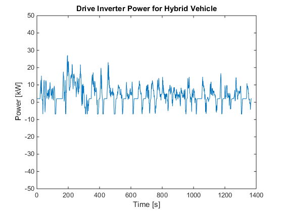
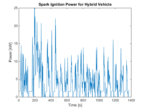
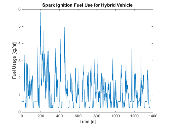
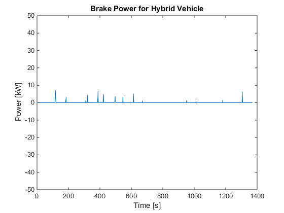
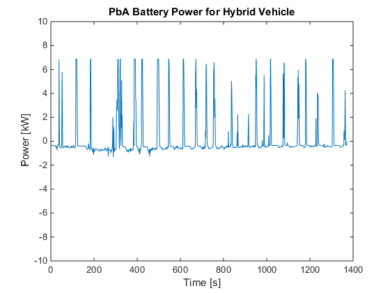
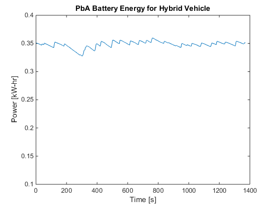
for i=1:k
    if Pm(i,1)<-6.875       %Inverter has a lower limit of -6.875 kW
        Pm(i,1)=-6.875;
    end
end
figure;
plot(Pm)
title('Drive Inverter Power for Hybrid Vehicle')
ylabel('Power [kW]')
xlabel('Time [s]')
axis([0 1400 -50 50])
figure;
plot(Pen)
title('Spark Ignition Power for Hybrid Vehicle')
ylabel('Power [kW]')
xlabel('Time [s]')
axis([0 1400 0 25])
figure;
plot(f)
title('Spark Ignition Fuel Use for Hybrid Vehicle')
ylabel('Fuel Usage [kg/hr]')
xlabel('Time [s]')
axis([0 1400 0 6])
figure;
plot(Pb)
title('Brake Power for Hybrid Vehicle')
ylabel('Power [kW]')
xlabel('Time [s]')
axis([0 1400 -50 50])
figure;
plot(Ps)
title('PbA Battery Power for Hybrid Vehicle')
ylabel('Power [kW]')
xlabel('Time [s]')
axis([0 1400 -10 10])
figure;
plot(E)
title('PbA Battery Energy for Hybrid Vehicle')
ylabel('Power [kW-hr]')
xlabel('Time [s]')
axis([0 1400 0.1 0.4])
Calculating optimal global fuel economy
%Integrating fuel consumption [g/s] to total fuel [g]
fuel=trapz(time,x(1:k,1));
%Integrating velocity [m/s] to total distance travelled [m]
distance=trapz(time,ve);
%Calculating distance travelled per total fuel consumed and converting to
%miles per gallon.
MPG=(distance*1000/fuel)*0.734/(0.2642*1609.34);
display(MPG)
MPG =

   44.6356
Solution for Internal Combustion Vehicle(without battery)
Generating equality constraint matrices
The solution for the internal combustion vehicle uses the same input
parameters and matrices and arrays as initialized above. The matrix
equality constraint Ax==b is made from the equality equations where A is
a 3*kx11*k matrix and b is a 3*kx1 matrix. Slack and surplus variables
were added to 2 equations to convert the inequality constraints into
equality constraints. Ax==b consists of 3 equations:


A=[T,-0.059.*T,-T,Z,Z;-T,0.096.*T,Z,T,Z;Z,T,Z,Z,-T];

b=zeros(3*k,1);                 %Initializing b
b(1:k,1)=0.075.*Onit;           %Equation 1 right side
b(k+1:2*k,1)=1.041667.*Onit;    %Equation 2 right side
b(2*k+1:3*k,1)=Pm;              %Equation 3 right side

c=zeros(1,5*k);
c(1,1:k)=one;
Generating inequality constraint matrices
The matrix inequality constraint Gx<=H is made from the inequality
equations where G is a 4*kx11*k matrix and H is a 4*kx1 matrix. The
inequality constraints consist of the upper bound limits on the two
parameters Pe, Pb, and upper bound limits on the engine slew rate. The
four inequality equations are as follows:

G=[Z,T,Z,Z,Z;Z,Z,Z,Z,T;Z,D,Z,Z,Z;Z,-D,Z,Z,Z];
H=[50.*Onit;23.125.*Onit;10.*Onit;20.*Onit];
CVX Code
With the additions of slack and surplus variables, the total number of
variables in the convex optimization problem is 6855 with 5 vectors
each with 1371 elements (the vectors are fuel consumption (f), engine
power (Pe), surplus variable (s1), slack variable (s2), brake power
(Pb)). The problem is a linear program optimization problem, therefore,
all of the variables must be positive.
cvx_begin
    variables x(5*k,1)
    minimize c*x
    subject to
        A*x==b
        G*x<=H
        x>=0
cvx_end
Calling SDPT3 4.0: 12339 variables, 2742 equality constraints
   For improved efficiency, SDPT3 is solving the dual problem.
------------------------------------------------------------

 num. of constraints = 2742
 dim. of linear var  = 12339
*******************************************************************
   SDPT3: Infeasible path-following algorithms
*******************************************************************
 version  predcorr  gam  expon  scale_data
    NT      1      0.000   1        0
it pstep dstep pinfeas dinfeas  gap      prim-obj      dual-obj    cputime
-------------------------------------------------------------------
 0|0.000|0.000|3.2e+02|1.1e+02|4.7e+09| 1.614504e+07  0.000000e+00| 0:0:00| spchol  1  1
 1|0.992|0.989|2.6e+00|1.2e+00|6.6e+07| 1.551967e+07 -4.639023e+06| 0:0:00| spchol  1  1
 2|1.000|1.000|3.1e-06|8.1e-03|9.4e+06| 6.813956e+06 -2.513010e+06| 0:0:00| spchol  1  1
 3|0.989|0.989|3.1e-06|4.1e-03|1.1e+05| 7.869150e+04 -2.645064e+04| 0:0:00| spchol  1  1
 4|0.938|0.956|2.1e-07|5.7e-04|6.1e+03| 6.698149e+03  6.562814e+02| 0:0:00| spchol  1  1
 5|0.789|0.935|4.4e-08|7.4e-05|3.9e+03| 4.987997e+03  1.067483e+03| 0:0:00| spchol  1  1
 6|0.911|0.905|4.0e-09|1.1e-05|4.7e+02| 2.654573e+03  2.187112e+03| 0:0:00| spchol  1  1
 7|0.977|0.873|2.8e-10|1.7e-06|1.1e+02| 2.381413e+03  2.267879e+03| 0:0:00| spchol  1  1
 8|0.963|0.982|9.0e-11|7.0e-08|2.3e+01| 2.321783e+03  2.299163e+03| 0:0:00| spchol  1  1
 9|0.946|0.873|4.0e-11|1.2e-08|2.3e+00| 2.305961e+03  2.303702e+03| 0:0:00| spchol  1  1
10|0.948|0.902|2.1e-12|1.6e-09|2.4e-01| 2.304662e+03  2.304420e+03| 0:0:00| spchol  1  1
11|0.977|0.979|4.8e-14|3.5e-11|5.8e-03| 2.304522e+03  2.304516e+03| 0:0:00| spchol  1  1
12|0.993|0.992|3.5e-16|1.3e-12|1.2e-04| 2.304519e+03  2.304519e+03| 0:0:00| spchol  1  1
13|0.996|0.994|1.7e-16|1.0e-12|1.8e-06| 2.304519e+03  2.304519e+03| 0:0:00|
  stop: max(relative gap, infeasibilities) < 1.49e-08
-------------------------------------------------------------------
 number of iterations   = 13
 primal objective value =  2.30451866e+03
 dual   objective value =  2.30451866e+03
 gap := trace(XZ)       = 1.80e-06
 relative gap           = 3.91e-10
 actual relative gap    = 3.81e-10
 rel. primal infeas (scaled problem)   = 1.69e-16
 rel. dual     "        "       "      = 1.01e-12
 rel. primal infeas (unscaled problem) = 0.00e+00
 rel. dual     "        "       "      = 0.00e+00
 norm(X), norm(y), norm(Z) = 3.7e+01, 1.2e+03, 2.1e+03
 norm(A), norm(b), norm(C) = 1.2e+02, 3.8e+01, 3.4e+03
 Total CPU time (secs)  = 0.18
 CPU time per iteration = 0.01
 termination code       =  0
 DIMACS: 3.2e-15  0.0e+00  4.5e-11  0.0e+00  3.8e-10  3.9e-10
-------------------------------------------------------------------

------------------------------------------------------------
Status: Solved
Optimal value (cvx_optval): +498.439
Renaming variables
f=x(1:k,1)*3.6;         %Fuel consumption [kg/hr]
Pen=x(k+1:2*k,1);       %Engine power [kW]
s1=x(2*k+1:3*k,1);      %Surplus variable
s2=x(3*k+1:4*k,1);      %Slack variable
Pb=x(4*k+1:5*k,1);      %Brake power [kW]
Visualization for Internal Combustion Vehicle(without battery)
Generating plots
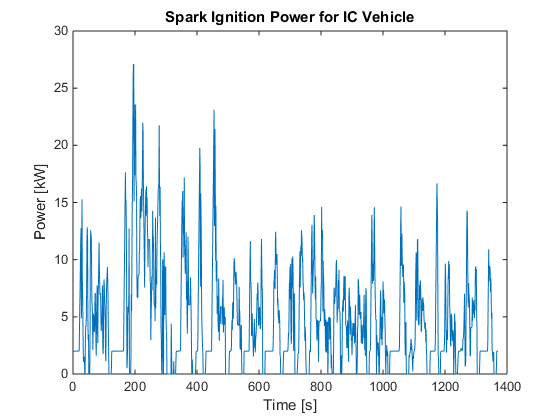
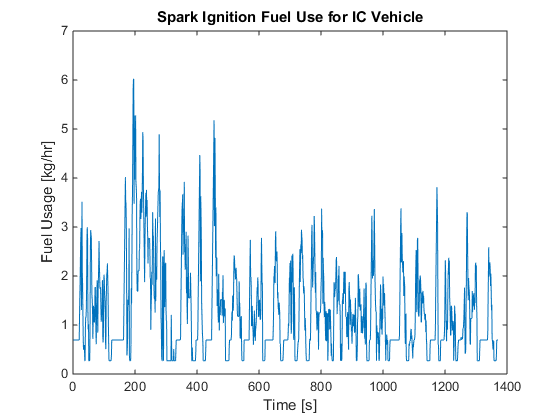
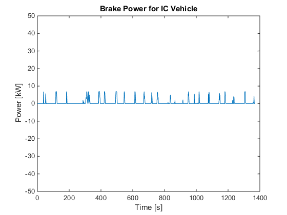
figure;
plot(Pen)
title('Spark Ignition Power for IC Vehicle')
ylabel('Power [kW]')
xlabel('Time [s]')
axis([0 1400 0 30])
figure;
plot(f)
title('Spark Ignition Fuel Use for IC Vehicle')
ylabel('Fuel Usage [kg/hr]')
xlabel('Time [s]')
axis([0 1400 0 7])
figure;
plot(Pb)
title('Brake Power for IC Vehicle')
ylabel('Power [kW]')
xlabel('Time [s]')
axis([0 1400 -50 50])
Calculating optimal global fuel economy
%Integrating fuel consumption [g/s] to total fuel [g]
fuel=trapz(time,x(1:k,1));
%Integrating velocity [m/s] to total distance travelled [m]
distance=trapz(time,ve);
%Calculating distance travelled per total fuel consumed and converting to
%miles per gallon.
IC_MPG=(distance*1000/fuel)*0.734/(0.2642*1609.34);
display(IC_MPG)
IC_MPG =

   41.5431
Analysis and Conclusions
   The code successfully reproduced the global fuel economy for both the
hybrid vehicle and the internal combustion vehicle. The authors had a
global fuel economy of 44.44 mpg and 41.55 mpg for the hybrid vehicle
and internal combustion vehicle, respectively. Whereas the reproduced
results were 44.64 mpg and 41.54 mpg for the hybrid and internal
combustion vehicles respectively. The percentage errors between the two
sets of results were 0.45% and 0.02%.
  The authors did not provide any graphs for the internal combustion
vehicle, however, they did provide graphs for the hybrid vehicle of the
drive inverter power, engine power, fuel usage, brake power, battery
power and battery energy. The reproduced graphs for the drive inverter
power and brake power closely matched the graphs given in the paper.
   The reproduced spark ignition power followed the same trend as the
given spark ignition power however the reproduced spark ignition power
values appeared to be greater than the given values by a factor of 0.25
for values greater than  approximately 10 kW. The reproduced spark
ignition fuel use also over predicted the given results by some vertical
offset and factor. Fromthese results, it is suspected that the
inequality equations relating fuel usage to spark ignition power given
in the paper were eithersubject to error or required further
modifications before implementing them in the linear program.
   The positive values of the reproduced battery power perfectly matched
the positive values of the given batterypower when an upper limit of
6.875 kW was applied.  Although an upper limit of 6.875 kW was not
explicitly given in the paper, it was implicity given from the given
inverter power graph. The graph shows that a maximum of 6.875 kW can be
regenerated from the vehicle's kinectic power. Therefore, due to the
inverter power upper limit, the battery can only accept 6.875 kW. The
negative battery power did not match the given negative battery power.
This occurred because the power supplied by the engine was nearly enough
to power the motor, brakes and auxiliary systems. The maximum power that
the battery had to supply was 1.3322 kW. The engine was capable of
supplying a maximum power of 50 kW, however, only a maximum of 26.875 kW
was used because the cost function was proportional to spark ignition
power (engine supply power).
   The battery energy had the same trend as the given battery energy,
however, the reproduced graph was different than the given graph because
the battery energy was dependent on the battery power.
   Although the plots of engine power and engine fuel use match with
those presented in the paper,its not the same in case of the plots of
battery power and energy and engine fuel use. So, we modified the limits
on battery energy,battery charge and discharge rates. For battery
maximum capacity of 0.4kW-hrs, maximum charge and discharge rates of
6.54kW and approximating the fuel consumption curve of the engine by:


We obtain all the plots similar to those presented in paper. However,
the global fuel optimal economy obtained after changing the values is
50.1mpg, with an error of 12% from the value mentioned by the
author (44.44mpg).
   Lastly, the code did not behave as the code described by the authors.
The code for the hybrid vehicle as reproduced in this project had 23306
variables and 6853 equality constraints. As recorded by Tate and Boyd,
their program had 26068 variables and 19210 constraints. The reproduced
code took 0.65 seconds to complete whereas Tate and Boyd reported their
code taking less than 2 minutes. These differences could be related to
the differing softwares used to execute the linear program. As stated
above, the reproduced code used CVX in Matlab while the original authors
used PCx in Pentium Pro.
References
[1] Tate, E. D. and Boyd, S. P.,2000, "Finding ultimiate limits of
performance for hybrid electric vehicles", _Future Transporation_
_Technology Conference_, 2000
[2] Michael Grant and Stephen Boyd. CVX: Matlab software for disciplined
convex programming, version 2.0 beta. http://cvxr.com/cvx, September
2013.
[3] Michael Grant and Stephen Boyd. Graph implementations for nonsmooth
convex programs, Recent Advances in Learning and Control (a tribute to
M. Vidyasagar), V. Blondel, S. Boyd, and H. Kimura, editors, pages
95-110, Lecture Notes in Control and Information Sciences, Springer,
2008. http://stanford.edu/~boyd/graph_dcp.html.
[4] EPA, United States Environmental Protection Agency, 2016, "Federal
Test Procedure Revisions," from https://www3.epa.gov/otaq/sftp.htm