ECE 602 - Optimization Project - Network Lasso: Clustering and Optimization in Large Graphs
by Côme Carquex and Laura McCrackin
Based on the paper by D. Hallac et al, Proceedings of the ACM SIGKDD, 2015.
Contents
Problem formulation
Introduction
The paper introduces the Network Lasso, which is a generalization of the group Lasso. Lasso means "Least Absolute Shrinkage and Selection Operator", and the idea behind it is to optimize an objective function while performing some regularization. The Network Lasso allows one to perform Clustering and Optimization on a network.
General Formulation
The problem is formulated on a graph,  . is defined as a set of vertices
  and edges
  .
.  . Each node
  has an associated variable
  , such that
  , with
  . Moreover, a convex cost function
  is associated to each node. Finally, each edge
  is given a weight
  .
.
The objective function that we would like to minimize is written as follows:
Since the objective function is convex, any convex solver could potentially solve it. However, for large networks, we would like to decouple the problem and solve it in parallel. This paper describes a method to do so.
Application to Network-Enhanced Classification
The application considered in this report is the use of the Network Lasso to enhance the classification accuracy of a network of Support Vector Machine (SVM) classifiers, as described in section 5.1 of the original paper.
A synthetic network is created, where each node has a SVM classifier, but not enough data points to accurately estimate the model parameters. At each node, the optimization variable represents the parameters of the statistical model -- in our case, the SVM classifier.  corresponds to the losses of the model, and the edges encourage the adjacent nodes to have close model parameters to connected nodes. In this way, the models will effectively borrow strength from their neighbours to improve their own classification performance.
We will discuss the specifics of this problem further in the sections that follow.
Work realized
In this report, we present the work realized to solve the previously defined problem. The two main components of this work are the following:
- Writing the distributed solver, which is based on the Alternating Method of Nultipliers (ADMM)
- Apply the Network Lasso to a network of SVM classifiers, and compare performance with a naive approach as a benchmark.
Proposed solution
Alternating Direction Method of Multipliers (ADMM)
The objective function  is minimized using the Alternating Direction Method of Multipliers (ADMM), a method used for distributed convex optimization.
The idea behind ADMM is to solve an equivalent problem, that can be decoupled and solved in a distributed fashion. This optimization problem can be written as:
This similar problem is solved by writing its augmented Lagrangian  , where
  is the dual variable and
  is a penalty parameter, the value of which does not change the optimal solution, but might influnce the convergence rate.
This problem can be solved iteratively, for each variable (x, z, u). Moreover, the update of each variable is separable and can be computed independently, for each node and edge respectively. The steps are as follows:

The algorithm stops when the primal residual and the dual residual are below a certain threshold. The primal residual is the difference between and  and the dual residual is the difference
  .
.
Regularization path
The parameter  is left undefined in the previous section. In order to estimate the optimal lambda, the regularization path can be computed as a function of . The advantage of using the regularization path is that the new optimal values when increasing will be close to the previous one, and therefore by initializing the algorithm with the values from the previous iteration, we can benefit from a "warm start" and save a significant amount of computation time.
Non-convex extension
The method is also extended to non convex regularization term of the form:  . The only difference in terms of calculations for solving this new optimization problem is the update equation for the z variable. Since the new problem created is non-convex, it should be noted that the optimal point found by the solver might not be the global minimum. We do not consider the non-convex formulation in our implementation.
Data source
This section describes the application of the Network Lasso to a network enhanced SVM classification. The dataset used is artificial and its construction is as follows:
First, N nodes are created, where each node represent a SVM classifier. These nodes are equally divided into 20 groups. Each group is assigned a classifier, characterized by a decision boundary ![$[a^T, a_0]$](project_main_eq07518591069348129012.png) . For each node, 25 samples
. For each node, 25 samples  are generated in
  , with labels given by
with a, w and  drawn independently from a normal distribution.
The links between nodes are established as follows:
- Two nodes in the same group have a 50% chance of being linked
- Two node from different clusters have a 1% chance of being linked
Solution
The parameters selected here generate a small network, to demonstrate results that are consistent with the paper in a short amount of time. A large network has been tested as well, and the results are included in the Results section.
% ====================
% = CODE STARTS HERE =
% ====================
clc;
clear all;
close all;
format long;
rng(0);                                 % for reproducibility

% % % % % % % % % % % % % % % % % % % % % % % % % % % % % % % % % % % % %
% DEFINE THE CONSTANT PARAMETERS
% % % % % % % % % % % % % % % % % % % % % % % % % % % % % % % % % % % % %


spaceDim = 4;                           % number of dimensions of the input space
nbGroup = 4;                            % number of groups
nbNodePerGroup = 5;                     % number of node per group
probaLinkIntraGroup = 0.5;              % probability of link between two nodes in the same group
probaLinkInterGroup = 0.01;             % probability of link between two nodes in two different groups
nbSamplePerNode = 25;                   % number of sample per node
c = 1;                                  % SVM soft margin parameter

% Calculate parameters based on the constants
nbNode = nbGroup * nbNodePerGroup;    % number of nodes in total

% % % % % % % % % % % % % % % % % % % % % % % % % % % % % % % % % % % % %
% GENERATE THE DATA
% % % % % % % % % % % % % % % % % % % % % % % % % % Put the first part into a pdf documents (better equation with full Latex)% % % % % % % % % % % %

[samples, y, a, a0] = generate_data(nbNode, nbSamplePerNode, nbGroup, spaceDim);
connection_matrix = generateConnectionMatrix(nbNode, nbGroup, probaLinkIntraGroup, probaLinkInterGroup);

% % % % % % % % % % % % % % % % % % % % % % % % % % % % % % % % % % % % %
% COMPUTE THE REGULARIZATION PATH
% % % % % % % % % % % % % % % % % % % % % % % % % % % % % % % % % % % % %

% For your convenience, we load a pre-run solution. To run the solver,
% uncomment the corresponding line (and comment out the load command).
load ADMM.mat
% [lambda, x_star] = ADMM_regularization_path(samples, y, c, connection_matrix, nbSamplePerNode);
Accuracy Calculations and Baseline Benchmark Result
In this section, we compute the average accuracy of the SVM at each node, based on new samples for testing. We also compute the accuracy of a baseline benchmark. This benchmark will be further discussed in the Analysis section.
nbTestSample = 200;
[accuracy] = classify_samples(x_star, a, a0, nbNode, nbGroup, nbNodePerGroup, nbTestSample, spaceDim);


% Compute the Baseline benchmark (explained in the Analysis section)

accuracy_benchmark = benchmark(samples, y, a, a0, connection_matrix, nbNode, nbSamplePerNode, nbNodePerGroup, nbGroup, nbTestSample, spaceDim, c);
Visualization of results
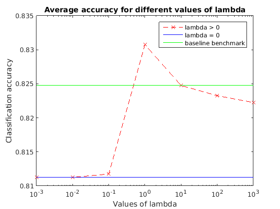
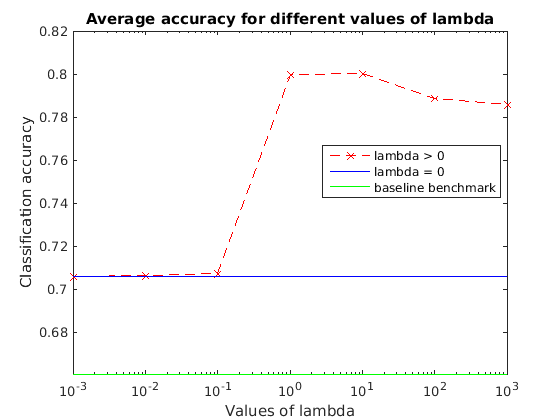
The following plot presents the accuracy results, computed for different cases. A case is defined by the constant parameters set at the beginning of the Solution section. We tried several different cases; large networks, as can be expected, take more time to converge.
The case corresponding to the parameters specified at the beginning of this code is given by the figure below:
figure(1);
semilogx(lambda(2:end), accuracy(2:end), '--xr'); hold on;
title('Average accuracy for different values of lambda');
xlabel('Values of lambda');
ylabel('Classification accuracy');
h1 = refline(0, accuracy(1));
h1.Color = 'b';
h2 = refline(0, accuracy_benchmark);
h2.Color = 'g';
legend('lambda > 0', 'lambda = 0', 'baseline benchmark');
hold off;
Results for other network parameters
Very Large Network
We ran the algorithm on a very large network (450 nodes, in  with 15 groups and 25 samples per node). The runtime was around 5 hours (single thread).
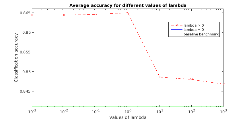
Very Small Network
When ran on a very small network (2 groups and 6 nodes in total), we obtained the regularization path below. The general trend of the graph is similar to the previous case, but with a different scale.
Analysis and Conclusion
The results are consistent with the paper
The results obtained are consistent with the results presented in the paper. We observe the improved performances given by the Network Lasso method compared to our simplified benchmarks.
The first benchmark (not included in the paper) consists of training each node's classifier using its own training points as well as the points from all its connected nodes. This is what we called the baseline benchmark .
The other benchmark is the case where  , where each node uses only its own samples.
We clearly see in each of the cases presented here the general trend of the regularization path -- improving until a  is reached, and then decreasing in performance until a
  has been reached, where all nodes can be considered to share the same classifier model.
In all cases tested, an optimal value which outperforms both benchmarks is found. It should be noted, however, that in many cases the difference between Network Lasso and the benchmarks is fairly small, and this small improvement may not always justify the significant increase in computational complexity.
Parallelization
In the original paper, the authors parallelized their solver using a 40-core machine. In our case, however, CVX is not parallelizable (CVX, by the way it is designed, cannot be run inside a parfor loop). For this reason, we use a reduced network size for our demonstration.
Learning experience
During this project, we learned about the ADMM algorithm, which is becoming increasingly popular for a wide variety of applications. We also learned how to implement a real optimization project and simple solver based on CVX.
Linked files
The following files are defined in the project:
ADMM Initialization and Steps
- ADMM_regularization_path.m: computes the regularization path
- x-step.m: performs the x step for a given node
- z-step.m: performs the z step for a given node
- u-step.m: performs the u step for a given node
- ADMM_convex_solver.m: performs the x, z, and u steps for each node
- node_solver.m: solves the SVM problem for a given node (used for our baseline benchmark and lambda=0)
Data generation and classification
- generate_data.m: generates the data points for the SVM classifier
- generateConnectionMatrix.m: generates the links between nodes for the network
- classify_samples.m: computes the classification accuracy of the Network lasso SVM
- benchmark.m: computes the baseline benchmark