ECE602 PROJECT: Tensor Completion for Estimating Missing Values in Visual Data Paper Review by Adam Sanderson
Contents
- 1. Description Of Problem
- 2. Common Functions and Notation in Paper
- 3. Code Initialization
- 4. Running Algorithms
- 5. CVX Completion
- 6. Simple Low Rank Tensor Completion(SiLRTC)
- 7. Fast Low Rank Tensor Completion(FaLRTC)
- 8. High Accuracy Low Rank Tensor Completion(HaLRTC)
- 9. Functions
- 10. Results
- 11. Conclusion
1. Description Of Problem
This paper creates algoritms estimate missing data in tensors by attempting to minimize the tensors rank. This problem can be formatted as...


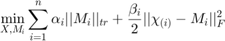
Where X is the new completed tensor/image, M is the starting image and  is a set containing known pixel/value indices. This cannot be readily solved as rank(X) is not a convex function. The trace norm is used to approximate the rank. This equation can be seen below.

 is the tensor trace norm which is formulated in section 2. This is then smoothed and some constraints are relaxed to make the 3 algorithms discussed below. In the paper these algorithms are explained via pseudo-code but as far as I am aware no code is available online to solve these problems.
I have attempted to use CVX to solve this problem but am unable to due to the vast amount of equations created when unfolding the Image in order to do tensor trace norm (explained in section 2). When attempting to use CVX I have experienced RAM usage of upwards of 20GB when solving a 60 by 60 RGB image Due to this limitation the report will focus on understanding and implementing the 3 algorithms developed in this paper and will not be using CVX.
2. Common Functions and Notation in Paper
Many of the functions used in this are similar to those taught in the course so some will be covered breifly. For simplicities sake  will be the tensor argument that we are trying to find and
  is a matrix.
  will be the tensor containing known values and is a set containing known pixel/value indices.
 is a matrix whose diagonal elements are the singular values of a matrix.
  is the value at
  .
.  is the singular value decomposition of .
The spectral norm is  or the largest singular value of a matrix.
 is the inner product of two tensors or matricies
The shrinkage operator is  .
.
Where  .
.
The truncate operator is  .
.
Where  .
.
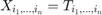
It is also common to unfold a tensor about its  dimension to create a matrix, this can be denoted as
 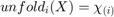 and the reverse operation fold is
  .
.
The trace norm of a tensor is defined as  .
.
Where  is the trace norm of a matrix and
  is a constant where
  and
and  .
.
 is the Frobenius norm.
3. Code Initialization
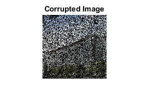
The code below is used to import the image into Matlab, generate known indices and create a corrupted version of the image.
rng('shuffle');

% Setting Variables and Importing Image
KnownPercentage = 50;
Image = imread('Thumb.jpg');
imshow(Image);
title('Original Image');
snapnow;
Image = double(Image);

% Corrupting Random Pixels
imSize = size(Image);
known = randperm(prod(imSize)/imSize(3), ...
    floor(KnownPercentage/100*(prod(imSize)/imSize(3))));
X = zeros(imSize);
X = double(ReplaceInd(X,known,Image,imSize));

imshow(uint8(X));
title('Corrupted Image');
4. Running Algorithms
SiLRTC(Image,500,known)
%CVXLRTC(Image,known)
FaLRTC(Image,50,known)
HaLRTC(Image,500,known)
5. CVX Completion
This algorithm was left in to show the general process of using CVX to solve the low rank tensor completion problem. This problem essentially tries to solve the very first minimization problem and reduce the trace norm of the unfolded corrupted image. It however cannot be run due to the large amount of variables created by CVX when solving the tensor trace norm of the unfolded corrupted Image. This process can create over 2^53 equations for CVX to solve even when using a small image.
function X = CVXLRTC(Image,known)

a = abs(randn(3,1));
a = a./sum(a);

cvx_begin

cvx_precision low

variable X(imSize)
f = 0;

f = a(1)*norm_nuc(unfold(X,1))+a(2)*norm_nuc(unfold(X,2))+a(3)*norm_nuc(unfold(X,3));

minimize (f)

subject to
for i = 1:length(known)
    [in1,in2] = FindInd(known(i),imSize);
    X(in1,in2,:) == Image(in1,in2,:);
end
cvx_end

imshow(uint8(X));
end
6. Simple Low Rank Tensor Completion(SiLRTC)
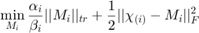
The idea behind SiLRTC is to break into multiple independant variables. The reason for doing this is that the trace norm of each unfolded matrix of the tensor X is somewhat independant from eachother. This new approach allows each Mi to be optimized indepentantly thus simplifying the problem. This turns the new problem into...


The equality restraints are then relaxed and this problem becomes...
Where  is a positive real value.
This algorithm is then solved via block coordinate descent. Essentially a group of variables will be solved while the other variables are fixed. These groups will be split into n + 1 blocks (each Mi and X) where n is the tensor order. The equation below must be solved to find X when each Mi is fixed.
The solution to this is given by...
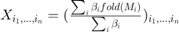 when
when 
 when
when 
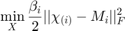
While the equation below must be solved to find each  when X and each other
  is fixed.
This can be shown to be solved by  when
when 
This is then solved by running  loops where each is solved and then is updated.
The basic algorithm is explained using the comments in the code below.
function SiLRTC(Image,K,known)
%assuming image is 3 dimensional
imSize = size(Image);

%Corrupting Image
X = zeros(imSize);
X = double(ReplaceInd(X,known,Image,imSize));

%Create random alphas and betas
b = abs(randn(3,1))/200;
a = abs(randn(3,1));
a = a./sum(a);

%main loop
for k = 0:K
    %initialize Mi's
    M = zeros(imSize);
    for i = 1:3
        %Create Mi's multiply by appropriate beta value
        %fold them and add into tensor get Mi values immediately into
        %tensor for so X can be updated
        M = M + Mfold(b(i)*shrinkage(unfold(X,i),a(i)/b(i)),i,imSize);
    end
    %Divide by sum of betas
    M = M./sum(b);

    %Update indices that we know from Image into M and set X equal to M
    M = ReplaceInd(M,known,Image,imSize);
    X = M;
end
%Ouput Image
imwrite(uint8(X),'html/SiFinal.jpg')

%Output Absolute Value Error Image
imwrite(uint8(abs(double(Image)-double(X))),'html/SiError.jpg')
end
7. Fast Low Rank Tensor Completion(FaLRTC)
To my knownlege this algorithm approaches solving the tensor norm problem, outlined in section 1, by solving a smoothed version and then using block gradient descent on the smoothed algorithm.
The smoothed algorithm is...
This function is solved by a modified gradient descent method. The gradient of the function above can be found to be...
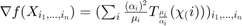 when
when
 when
when
I was unable to find a good way to calculate the objective function f(X) so I used the unsmoothed objective function, the trace norm, to simplify my calculations. The original plan was to put the function into CVX and solve the maximize problems, but due to the amount of variables introduced and number of itterations it was far too slow to be used. Even with the simplified objective function this algorithm still works very well.
The basic algorithm is explained using the comments in the code below
function FaLRTC(Image,K,known)
%assuming image is 3 dimensional
imSize = size(Image);

%Corrupting Image
X = zeros(imSize);
X = double(ReplaceInd(X,known,Image,imSize));

%Create needed constants and holder variables
a = abs(randn(3,1));
a = a./sum(a);
C = 0.5;
u = 10^5;
ui = a./u;
Z = X;
W = X;
B = 0;
L = sum(ui);
for k = 0:K
    while true
        Theta = (1+sqrt(1+4*L*B)) / (2*L);
        W = Theta/(B+Theta) * Z + B/(B+Theta) * X;

        %Compute f(x), f(w) and f'(w).
        dfw = zeros(imSize);
        fx = 0;
        fw = 0;

        for i = 1:3
            [Sig,T] = Trimming(unfold(X,i),ui(i)/a(i));
            fx = fx + sum(Sig(:));
            [Sig,T] = Trimming(unfold(W,i),ui(i)/a(i));
            fw = fw + sum(Sig(:));
            dfw = dfw + Mfold(a(i)^2/ui(i)*T,i,imSize);
        end
        dfw = ReplaceInd(dfw,known,zeros(imSize),imSize);

        %If step size is too low then break
        if fx <= fw - sum(dfw(:).^2)/L
            break;
        end

        %Solve for new f(X) using modified W matrix
        Xp = W - dfw/L;
        fxp = 0;
        for i = 1:3
            [Sig,T] = Trimming(unfold(Xp,i),ui(i)/a(i));
            fxp = fxp + sum(Sig(:));
        end

        %If step size is not too large update and break
        if fxp <= fw - sum(dfw(:).^2)/2/L
            X = Xp;
            break;
        end

        %Update L and rerun
        L = L/C;

        %If L is too large throw error and exit
        if L == Inf
            disp('Error')
            imwrite(uint8(X),'html/FaFinal.jpg')
            exit
        end
    end

    % Update Z and B
    Z = Z - Theta*dfw;
    B = B + Theta;
end
%Output Image
imwrite(uint8(X),'html/FaFinal.jpg')

%Output Absolute Value Error Image
imwrite(uint8(abs(double(Image)-double(X))),'html/FaError.jpg')
end
8. High Accuracy Low Rank Tensor Completion(HaLRTC)
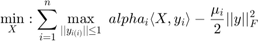
This algorithm utilizes alternating direction method of multipliers (ADMM) framework to solve this problem. In this case the algorithm is formulated as follows.
Where  are tensors.
A modified Lagrandian is then defined where...

These can then be updated by...
1) 
2) 
3) 
for step 1 the solution can be given by...

step 2
 when .
when .
step 3 is already in an easily solvable form.
The basic algorithm is explained using the comments in the code below.
function HaLRTC(Image,K,known)
%assuming image is 3 dimensional
imSize = size(Image);

%Corrupting Image
X = zeros(imSize);
X = double(ReplaceInd(X,known,Image,imSize));

%Setup alpha and rho values
a = abs(randn(3,1));
a = a./sum(a);
p = 1e-6;

%Create tensor holders for Mi and Yi done to simplify variable storage

ArrSize = [imSize,ndims(Image)];
Mi = zeros(ArrSize);
Yi = zeros(ArrSize);

%Main Loop
for k = 0:K

    %Calculate Mi tensors (Step 1)
    for i = 1:3
        Mi(:,:,:,i) = Mfold(shrinkage(unfold(X,i) ...
            + unfold(squeeze(Yi(:,:,:,i)),i)./p,a(i)/p),i,imSize);
    end

    %Update X (Step 2)
    X = (sum(Mi-Yi./p,4))/3;
    X = ReplaceInd(X,known,Image,imSize);

    %Update Yi tensors (Step 3)
    for i = 1:ArrSize(length(ArrSize))
        Yi(:,:,:,i) =  squeeze(Yi(:,:,:,i))-p*(squeeze(Mi(:,:,:,i))-X);
    end

    %Modify rho to help convergence
    p = 1.2*p;
end
%Output Image
imwrite(uint8(X),'html/HaFinal.jpg')

%Output Absolute Value Error Image
imwrite(uint8(abs(double(Image)-double(X))),'html/HaError.jpg')
end
9. Functions
The functions below are calculations that need to be done repeatedly in each algorithm. Most of them work perfectly, however some may need to be updated in order to function if a tensor that is not 3rd order is put into this system. The functions ReplaceInd, FindInd, unfold and Mfold rely on a 3rd order tensor being used.
The ReplaceInd function is used to replace values at certain indices with values from another tensor at the same index. This is used to simplify calculations where we need to update only values that are not known , instead of going index by index they are all updated and then the known values are put back in.
FindInd takes an array of numbers and correlates it to an indices to be replaced, this was done to simplify the generation of pixels to be removed.
The unfold and Mfold functions both do as described in section 2. They fold a matrix into a tensor and unfold a tensor into a matrix depending on the mode of the tensor that we wish to unfold.
Trimming and shrinkage both do as described in section 2.
function mOut = ReplaceInd(X,known,Image,imSize)
for i = 1:length(known)
    [in1,in2] = FindInd(known(i),imSize);
    X(in1,in2,:) = double(Image(in1,in2,:));
end
mOut = X;
end

function [a,b] = FindInd(num,mSize)
a = ceil(num/mSize(2));
b = mSize(1) - mod(num,mSize(1));
end

function D = shrinkage(X,t)
[U,Sig,V] = svd(X,'econ');
for i = 1:size(Sig,1)
    Sig(i,i) = max(Sig(i,i)-t,0);
end
D = U*Sig*V';
end

function [Sig,T] = Trimming(X,t)
[U,Sig,V] = svd(X,'econ');
SigT = Sig;
for i = 1:size(SigT,1)
    SigT(i,i) = min(SigT(i,i),t);
end
T = U*SigT*V';
end

function b = unfold(a,i)
b = [];
for j = 1:size(a,i)
    switch i
        case 1
            b = [b;vec(a(j,:,:))'];
        case 2
            b = [b;vec(a(:,j,:))'];
        case 3
            b = [b;vec(a(:,:,j))'];
    end
end
end


function c = Mfold(a,i,OrDim)
c = [];
for j = 1:OrDim(i)
    switch i
        case 1
            c(j,:,:) = reshape(a(j,:),OrDim(2),OrDim(3));
        case 2
            c(:,j,:) = reshape(a(j,:),OrDim(1),OrDim(3));
        case 3
            c(:,:,j) = reshape(a(j,:),OrDim(1),OrDim(2));
    end
end
end
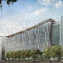
10. Results
The results of the algoritms can be seen below. These tests were done with 50% of the image's pixels removed/corrupted. It can be seen that SiLRTC, FaLRTC and HaLRTC all do a very good job at filling in missing values. However, the amount of cycles needed to fill in the values are vastly different. In the example image chosen, FaLRTC as the name implies is able to get an adequate solution through very few itterations. SiLRTC and HaLRTC require far more to produce meaningful results. This may just be due to the nature of the image chosen. It is rather low resolution and the image has many complicated areas so it is may be difficult to reduce the rank of this image.
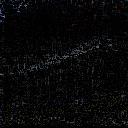
I am also disappointed with the output image from the HaLRTC algorithm compared to SiLRTC. Somehow the high accuracy algorithm managed to be matched by the the simple one. The absolute value difference images below are a good metric for the performance of each of these algorithms. It can be seen that the algorithms performed similarly through the number of cycles was different. This may be caused by the stucture of the image, the choices of constants, the number of itterations performed, and/or by the amount of corrupted data. When there is a lower percentage of data available HaLRTC tends to perform better than the other algorithms.
SiLRTC

Absolute Value Difference SiLRTC - Original

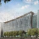
FaLRTC
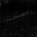
Absolute Value Difference FaLRTC - Original
HaLRTC
Absolute Value Difference HaLRTC - Original
11. Conclusion
Overall these are incredibly useful algorithms and the results have been astounding. I have found that there can be serious difficulty in finding proper  ,
,  and
and  values. It is also difficult to find the number of iterations to run. The algorithms tend to remove outliers from the data. This can cause issues with certain images; such as the one used as a sample in this report. It tends to be more effective in images with some form of uniformity or with outliers purposely removed.