ECE602 Project: A Robust Maximin Approach for MIMO Communications With Imperfect Channel State Information Based on Convex Optimization [1]
Student Name: ALONG JIN (20687178)
Contents
- 1. Background of MIMO Systems and Related Work
- 2. System Model and Problem Formulation
- 3. Solving the Proposed Maximin Problem
- 4. Convex Uncertainty Regions
 4-1. Estimation Gaussian Noise
- 4-2. Quantization Error
- 4-3. Combined Estimation and Quantization Errors
- 5. Repreducing Simulation Results
- 5-1. Mean Value of Normalized Power Allocation (Gaussian Noise with Spherical Uncertainty Regions)
- 5-2. Mean Value of Minimum Transmit Power (dB) - TDD System - Spherical Uncertainty Regions
- 5-3. Mean Value of Minimum Transmit Power (dB) - FDD System - Cubic Uncertainty Regions
- 5-4. Probability of Service Provision (Gaussian Noise with Spherical Uncertainty Regions)
- 5-5. Probability of Service Provision (Quantization Error with Cubic Uncertainty Regions)
- 6. Concluding Remarks
- 7. Reference
1. Background of MIMO Systems and Related Work
The multiple-input-multiple-output (MIMO) systems have been widely studied and used to achieve the spatial diversity and improve the quality of wireless communications. The performance of MIMO systems depend heavily on the quantity and quality of the channel state information (CSI) at both the transmitters and receivers, and such channel knowledge is generally imperfect in realistic scenarios.
Let the  be the estimation of the imperfect channel. In the non-robust design, only the maximum eigenmode of
  is used. On the other hand, the pure orthogonal space-time block code (OSTBC) approach uses all the eigenmodes, over which the transmit power is uniformly allocated. However, without taking into account explicitly the errors in the CSI estimation, both the non-robust and pure OSTBC systems suffer from severe performance degradation with increasing error level.
In this paper, the authors propose a robust design for MIMO communication system by explicitly considering the errors in the channel estimate. Particularly, the robust design is based on the notion of maximin philosophy. The authors first give the system model and formulate an maximin problem. Then, by assuming the convex uncertainty regions of the errors, the optimization problem is transformed to a simple convex problem. Besides, different convex uncertainty regions are investigated, in terms of the Gaussian noise and quantization error.
2. System Model and Problem Formulation
Consider a MIMO system with  transmit and
  receive antennas, where the actual channel matrix is
  . Let
. Let  be the error in the estimate, there is

To design robust transmitter, the authors adopt OSTBC block and distribute transmit power over the all the eigenmodes of . Let ![$\mathrm{\hat{U}} = [\mathrm{\hat{u}_1} \cdots \mathrm{\hat{u}_{n_T}}]$](mainOPT_eq16746043636476447498.png) be the normalized eigenvectors of
be the normalized eigenvectors of  , and the corresponding power allocation be
 ![$\mathbf{p}^T = [p_1 \cdots p_{n_T}]$](mainOPT_eq15576271220262090610.png) . The performance of proposed system can be measured by the SNR, given by
. The performance of proposed system can be measured by the SNR, given by
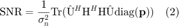
where  is the power of additive white Gaussian noise (AWGN) at the receiver. Based on this, the performance function
  in this system can be defined as

The objective is to optimize the power allocation  with the worst case error in the uncertainty region
  . Then, the robust approach is formulated as

3. Solving the Proposed Maximin Problem
Assuming that the constraint set is convex, the maximin problem in (4) can be transformed into the following simplified convex optimization problem

where  is a dummy variable. The optimal robust power allocation
 ![$\mathbf{p}^* = [p_1^* \cdots p_{n_T}^*]^T$](mainOPT_eq14405696873299066835.png) is closely related to the optimal dual variables
is closely related to the optimal dual variables  associated with the convex optimization problem in (5), i.e.,
  .
.
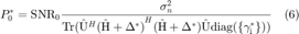
It should be noted that the optimal dual variables and worst case error  do not depend on the power budget
  . Thus, to achieve a target
  , the minimum transmit power is given by
4. Convex Uncertainty Regions
In the following, two sources of errors are identified and described, as well as the joint uncertainty region.
4-1. Estimation Gaussian Noise
Let the unbiased channel estimation be  , where
  is the zero-mean estimation noise, independent from . If the channel matrix and error matrix have i.i.d. components with zero-mean and variance
  and
and  , respectively, the uncertainty region for the channel estimation reduces to a sphere of radius
  , given by
where  . Denote
  , which is the probability of providing required QoS, i.e., probability of having a SNR higher than the target . The relationship between
  and
and  is given by

where  is the cumulative density function of the chi-square distribution with
  degrees of freedom.
Besides, for spherical uncertainty regions, a closed-form solution is provided, as shown in the subsection IV-E of the paper [1].
4-2. Quantization Error
Due to finite capacity of feedback channel, the channel response has to be quantized. Assuming that uniform quantization is used with the step  , the quantization SNR is defined as
  . The uncertainty region for the channel estimation is a hypercube centered at , given by
![$$ \mathcal{R} = \{ \Delta: |\mathrm{Re}\{[\Delta]_{ij}\}| \le
\frac{\Delta_q}{2}, ~|\mathrm{Im}\{[\Delta]_{ij}\}| \le
\frac{\Delta_q}{2} \} \quad (9) $$](mainOPT_eq08267280054663197415.png)
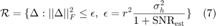
4-3. Combined Estimation and Quantization Errors
In realistic scenarios, both Gaussian noise and quantization error effect the channel estimation. Thus, an appropriate uncertainty region for the errors can be defined as
![$$ \mathcal{R} = \{ \Delta = \Delta_1 + \Delta_2: ||\Delta_1||_F^2 \le
\epsilon, ~|\mathrm{Re}\{[\Delta_2]_{ij}\}| \le \frac{\Delta_q}{2},
~|\mathrm{Im}\{[\Delta_2]_{ij}\}| \le \frac{\Delta_q}{2} \} \quad (10) $$](mainOPT_eq07575814766028597394.png)
According to the region, the optimization problem in (5) can be rewritten as the following convex quadratic problem:
![$$ \min_{t, \Delta_1, \Delta_2} t \quad \mathrm{s.t.} \quad t \ge P_0
\mathrm{\hat{u}_i}^H \mathrm{(\hat{H} + \Delta_1 + \Delta_2)}^H
\mathrm{(\hat{H} + \Delta_1 + \Delta_2)} \mathrm{u_i} ~~\forall i, \quad
\mathrm{Tr}(\Delta_1^H \Delta_1) \le \epsilon, \quad
|\mathrm{Re}\{[\Delta_2]_{ij}\}| \le \frac{\Delta_q}{2}, \quad
|\mathrm{Im}\{[\Delta_2]_{ij}\}| \le \frac{\Delta_q}{2} \quad (11) $$](mainOPT_eq18075498585191073993.png)
5. Repreducing Simulation Results
In the following, the main results in the paper [1] will be reproduced with CVX in MATLAB.
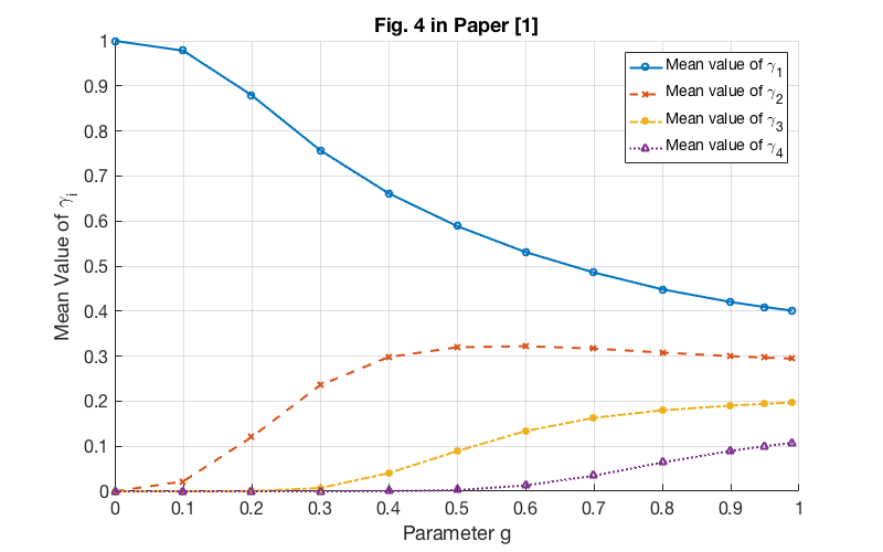
5-1. Mean Value of Normalized Power Allocation (Gaussian Noise with Spherical Uncertainty Regions)
close all;
clear all;
%
% Parameters
varH = 2; % variance of channel matrix H
varE = 1; % variance of error matrix E
nT = 4; % number of transmit antennas
nR = 6; % number of receiver antennas
g = 0:0.1:0.9;
g = [g 0.95 0.99]; % parameter g
%
% Optimization problem with CVX (Eq.(23) in paper)
N = 300; % number of iterations
pDist = zeros(nT,12); % normalized power allocation for different radius
for a = 1:N
  H = (randn(nR,nT) + i*randn(nR,nT))*sqrt(varH/2); % actual CSI matrix
  E = (randn(nR,nT) + i*randn(nR,nT))*sqrt(varE/2); % estimation error matrix
  estH = (H+E)*varH/(varH+varE); % estimated CSI matrix
  [U, ~] = eig(estH'*estH); % normalized eigenvectors and eigenvalues (ascending order)
  r = norm(estH(:))*g; % radius of spherical uncertainty region
  for b = 1:12
      cvx_begin
          variable t;
          variable delta(nR,nT) complex;
          dual variables gamma{nT};
          minimize (t);
          norm(delta(:)) <= r(b);
          for c = 1:nT
              gamma{c} : t >= quad_form((estH+delta)*U(:,c), diag(ones(nR,1)));
          end
      cvx_end
      pDist(:,b) = pDist(:,b)+cell2mat(gamma);
  end
end
pDist = pDist/N; % mean value of normalized power allocation
save('data/powerDist', 'g', 'pDist'); % save data
% Fig.4 in Paper [1]
load('data/powerDist');
fig = figure;
set(fig, 'Units', 'Pixels', 'Position', [100 600 800 500]);
set(gca, 'Fontsize', 16);
hold on;
grid on;
plot(g, pDist(4,:), '-o', g, pDist(3,:), '--x', g, pDist(2,:), '-.*', g, pDist(1,:), ':^', 'linewidth', 2);
legend('Mean value of \gamma_1', 'Mean value of \gamma_2', 'Mean value of \gamma_3', 'Mean value of \gamma_4');
xlabel('Parameter g');
ylabel('Mean Value of \gamma_i');
title('Fig. 4 in Paper [1]');

% Code: powerDist.m
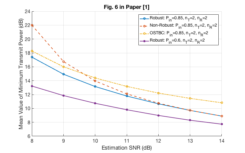
5-2. Mean Value of Minimum Transmit Power (dB) - TDD System - Spherical Uncertainty Regions
close all;
clear all;
%
% Parameters
SNR0 = 10; % target SNR
varG = 1; % variance of AWGN at receiver
varH = 2; % variance of channel matrix
estSNRdB = 8:14; % estimation SNR (dB)
estSNR = 10.^(estSNRdB/10); % estimation SNR
nT = 2; % number of transmit antennas
nR = 2; % number of receive antennas
%
% Algorithms
P0 = zeros(4,7); % minimum required transmit power
N = 2; % number of iterations
for a = 1:N
  H = (randn(nR,nT) + i*randn(nR,nT))*sqrt(varH/2); % actual CSI matrix
  E = randn(nR,nT) + i*randn(nR,nT); % estimation error matrix without specifying variance
  %
  qosP = 0.85; % probability of providing required QoS
  r = sqrt(chi2inv(qosP, 2*nR*nT)*varH./(1+estSNR)); % radius of spherical uncertainty region
  for b = 1:7
      varE = varH/estSNR(b); % variance of error matrix
      estH = (H+E*sqrt(varE/2))*varH/(varH+varE); % estimated CSI matrix
      [U, ~] = eig(estH'*estH); % normalized eigenvectors and eigenvalues (ascending order)
      %
      % Robust with all eigenmodes
      cvx_begin
          variable t;
          variable delta(nR,nT) complex;
          dual variables gamma{nT}; % dual variables
          minimize (t);
          norm(delta(:)) <= r(b);
          for c = 1:nT
              gamma{c} : t >= quad_form((estH+delta)*U(:,c), diag(ones(nR,1)));
          end
      cvx_end
      P0(1,b) = P0(1,b)+SNR0*varG/real(cell2mat(gamma)'*diag(U'*(estH+delta)'*(estH+delta)*U));
      %
      % Non-robust with maximum eigenmode
      cvx_begin
          variable delta(nR,nT) complex;
          minimize (norm((estH+delta)*U(:,nT), 'fro'));
          norm(delta(:)) <= r(b);
      cvx_end
      P0(2,b) = P0(2,b)+SNR0*varG/real(cvx_optval^2);
      %
      % OSTBC with equal power over all eigenmodes
      cvx_begin
          variable delta(nR,nT) complex;
          f = 0;
          for c = 1:nT
              f = f+quad_form((estH+delta)*U(:,c), diag(ones(nR,1)))/nT;
          end
          minimize (f);
          norm(delta(:)) <= r(b);
      cvx_end
      P0(3,b) = P0(3,b)+SNR0*varG/real(cvx_optval);
  end
  %
  % Robust for qosP = 0.6
  qosP = 0.6; % probability of providing required QoS
  r = sqrt(chi2inv(qosP, 2*nR*nT)*varH./(1+estSNR)); % radius of spherical uncertainty region
  for b = 1:7
      varE = varH/estSNR(b); % variance of error matrix
      estH = (H+E*sqrt(varE/2))*varH/(varH+varE); % estimated CSI matrix
      [U, ~] = eig(estH'*estH); % normalized eigenvectors and eigenvalues (ascending order)
      cvx_begin
          variable t;
          variable delta(nR,nT) complex;
          dual variables gamma{nT}; % dual variables
          minimize (t);
          norm(delta(:)) <= r(b);
          for c = 1:nT
              gamma{c} : t >= quad_form((estH+delta)*U(:,c), diag(ones(nR,1)));
          end
      cvx_end
      P0(4,b) = P0(4,b)+SNR0*varG/real(cell2mat(gamma)'*diag(U'*(estH+delta)'*(estH+delta)*U));
  end
end
P0 = 10*log10(P0/N); % minimum required transmit power (dB)
save('data/minPowerTDD.mat', 'estSNRdB', 'P0'); % save data
% Fig. 6 in Paper [1]
load('data/minPowerTDD');
fig = figure;
set(fig, 'Units', 'Pixels', 'Position', [100 600 800 500]);
set(gca, 'Fontsize', 16);
hold on;
grid on;
plot(estSNRdB, P0(1,:), '-o', estSNRdB, P0(2,:), '--o', estSNRdB, P0(3,:), '-.o', estSNRdB, P0(4,:), '-*', 'linewidth', 2);
legend('Robust: P_{in}=0.85, n_T=2, n_R=2', 'Non-Robust: P_{in}=0.85, n_T=2, n_R=2', ...
    'OSTBC: P_{in}=0.85, n_T=2, n_R=2', 'Robust: P_{in}=0.6, n_T=2, n_R=2');
xlabel('Estimation SNR (dB)');
ylabel('Mean Value of Minimum Transmit Power (dB)');
title('Fig. 6 in Paper [1]');

% Code: minPowerTDD.m
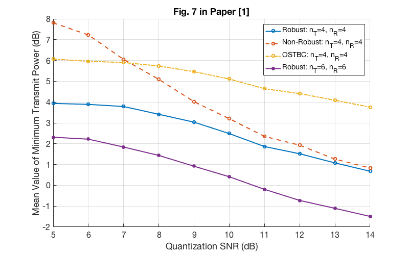
5-3. Mean Value of Minimum Transmit Power (dB) - FDD System - Cubic Uncertainty Regions
close all;
clear all;
%
% Parameters
SNR0 = 10; % target SNR
varG = 1; % variance of AWGN at receiver
varH = 2; % variance of channel matrix
qSNRdB = 5:14; % quantization SNR (dB)
qSNR = 10.^(qSNRdB/10); % quantization SNR
qSTEP = sqrt(6*varH./qSNR); % quantization step
%
% Algorithms
P0 = zeros(4,10); % minimum required transmit power
N = 300; % number of iterations
for a = 1:N
  nT = 4; % number of transmit antennas
  nR = 4; % number of receive antennas
  H = (randn(nR,nT) + i*randn(nR,nT))*sqrt(varH/2); % actual CSI matrix
  for b = 1:10
      estH = qSTEP(b).*round(H./qSTEP(b)); % estimated CSI matrix
      [U, ~] = eig(estH'*estH); % normalized eigenvectors and eigenvalues (ascending order)
      %
      % Robust with all eigenmodes
      cvx_begin
          variable t;
          variable delta(nR,nT) complex;
          dual variables gamma{nT}; % dual variables
          minimize (t);
          max(abs(real(delta(:)))) <= qSTEP(b)/2;
          max(abs(imag(delta(:)))) <= qSTEP(b)/2;
          for c = 1:nT
              gamma{c} : t >= quad_form((estH+delta)*U(:,c), diag(ones(nR,1)));
          end
      cvx_end
      P0(1,b) = P0(1,b)+SNR0*varG/real(cell2mat(gamma)'*diag(U'*(estH+delta)'*(estH+delta)*U));
      %
      % Non-robust with maximum eigenmode
      cvx_begin
          variable delta(nR,nT) complex;
          minimize (norm((estH+delta)*U(:,nT), 'fro'));
          max(abs(real(delta(:)))) <= qSTEP(b)/2;
          max(abs(imag(delta(:)))) <= qSTEP(b)/2;
      cvx_end
      P0(2,b) = P0(2,b)+SNR0*varG/real(cvx_optval^2);
      %
      % OSTBC with equal power over all eigenmodes
      cvx_begin
          variable delta(nR,nT) complex;
          f = 0;
          for c = 1:nT
              f = f+quad_form((estH+delta)*U(:,c), diag(ones(nR,1)))/nT;
          end
          minimize (f);
          max(abs(real(delta(:)))) <= qSTEP(b)/2;
          max(abs(imag(delta(:)))) <= qSTEP(b)/2;
      cvx_end
      P0(3,b) = P0(3,b)+SNR0*varG/real(cvx_optval);
  end
  %
  % Robust for nT = 6 and nR = 6
  nT = 6; % number of transmit antennas
  nR = 6; % number of receive antennas
  H = (randn(nR,nT) + i*randn(nR,nT))*sqrt(varH/2); % actual CSI matrix
  for b = 1:10
      estH = qSTEP(b).*round(H./qSTEP(b)); % estimated CSI matrix
      [U, ~] = eig(estH'*estH); % normalized eigenvectors and eigenvalues (ascending order)
      cvx_begin
          variable t;
          variable delta(nR,nT) complex;
          dual variables gamma{nT}; % dual variables
          minimize (t);
          max(abs(real(delta(:)))) <= qSTEP(b)/2;
          max(abs(imag(delta(:)))) <= qSTEP(b)/2;
          for c = 1:nT
              gamma{c} : t >= quad_form((estH+delta)*U(:,c), diag(ones(nR,1)));
          end
      cvx_end
      P0(4,b) = P0(4,b)+SNR0*varG/real(cell2mat(gamma)'*diag(U'*(estH+delta)'*(estH+delta)*U));
  end
end
P0 = 10*log10(P0/N); % minimum required transmit power (dB)
save('data/minPowerFDD.mat', 'qSNRdB', 'P0'); % save data
% Fig.7 in Paper [1]
load('data/minPowerFDD');
fig = figure;
set(fig, 'Units', 'Pixels', 'Position', [100 600 800 500]);
set(gca, 'Fontsize', 16);
hold on;
grid on;
plot(qSNRdB, P0(1,:), '-o', qSNRdB, P0(2,:), '--o', qSNRdB, P0(3,:), '-.o', qSNRdB, P0(4,:), '-*', 'linewidth', 2);
legend('Robust: n_T=4, n_R=4', 'Non-Robust: n_T=4, n_R=4', 'OSTBC: n_T=4, n_R=4', 'Robust: n_T=6, n_R=6');
xlabel('Quantization SNR (dB)');
ylabel('Mean Value of Minimum Transmit Power (dB)');
title('Fig. 7 in Paper [1]');

% Code: minPowerFDD.m
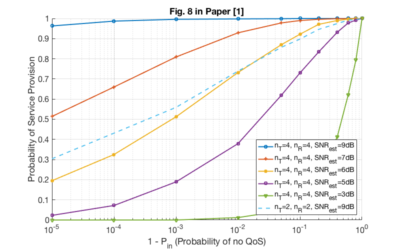
5-4. Probability of Service Provision (Gaussian Noise with Spherical Uncertainty Regions)
close all;
clear all;
%
% Parameters
varH = 2; % variance of channel matrix
noQoS = [0.00001 0.0001 0.001 0.01 0.05 0.1 0.2 0.4 0.6 0.8 1.0]; % probability of no QoS
qosP = 1 - noQoS; % probability of providing required QoS
estSNRdB = [9 7 6 5 3]; % estimation SNR (dB)
estSNR = 10.^(estSNRdB/10); % estimation SNR
varE = varH./estSNR; % variance of error matrix
%
% Algorithms
N = 1000; % number of iterations
pSev = N*ones(6,11); % number of service provision
for a = 1:N
  nT = 4; % number of transmit antennas
  nR = 4; % number of receive antennas
  H = (randn(nR,nT) + i*randn(nR,nT))*sqrt(varH/2); % actual CSI matrix
  E = randn(nR,nT) + i*randn(nR,nT); % estimation error matrix without specifying variance
  for b = 1:5
      estH = (H+E*sqrt(varE(b)/2))*varH/(varH+varE(b)); % estimated CSI matrix
      r = sqrt(chi2inv(qosP, 2*nR*nT)*varH./(1+estSNR(b))); % radius of spherical uncertainty region
      c = (norm(estH(:)) <= r);
      pSev(b,c) = pSev(b,c)-1; % actual CSI matrix H=0 belongs to the uncertainty region
  end
  %
  nT = 2; % number of transmit antennas
  nR = 2; % number of receive antennas
  H = (randn(nR,nT) + i*randn(nR,nT))*sqrt(varH/2); % actual CSI matrix
  E = (randn(nR,nT) + i*randn(nR,nT))*sqrt(varE(1)/2); % estimation error matrix
  estH = (H+E)*varH/(varH+varE(1)); % estimated CSI matrix
  r = sqrt(chi2inv(qosP, 2*nR*nT)*varH./(1+estSNR(1))); % radius of spherical uncertainty region
  b = (norm(estH(:)) <= r);
  pSev(6,b) = pSev(6,b)-1; % actual CSI matrix H=0 belongs to the uncertainty region
end
pSev = pSev/N; % probability of service provision
save('data/probServiceTDD.mat', 'noQoS', 'pSev'); % save data
% Fig.8 in Paper [1]
load('data/probServiceTDD');
fig = figure;
set(fig, 'Units', 'Pixels', 'Position', [100 600 800 500]);
hold on;
grid on;
plot(noQoS, pSev(1,:), '-o', noQoS, pSev(2,:), '-+', noQoS, pSev(3,:), '-*', 'linewidth', 2);
plot(noQoS, pSev(4,:), '-s', noQoS, pSev(5,:), '-v', noQoS, pSev(6,:), '--', 'linewidth', 2);
set(gca, 'XScale', 'log', 'Fontsize', 16);
legend('n_T=4, n_R=4, SNR_{est}=9dB', 'n_T=4, n_R=4, SNR_{est}=7dB', ...
    'n_T=4, n_R=4, SNR_{est}=6dB', 'n_T=4, n_R=4, SNR_{est}=5dB', ...
    'n_T=4, n_R=4, SNR_{est}=3dB', 'n_T=2, n_R=2, SNR_{est}=9dB', 'location', 'southeast');
xlabel('1 - P_{in} (Probability of no QoS)');
ylabel('Probability of Service Provision');
title('Fig. 8 in Paper [1]');

% Code: probServiceTDD.m
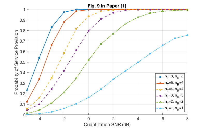
5-5. Probability of Service Provision (Quantization Error with Cubic Uncertainty Regions)
close all;
clear all;
%
% Parameters
varH = 2; % variance of channel matrix
qSNRdB = -5:8; % quantization SNR (dB)
qSNR = 10.^(qSNRdB/10); % quantization SNR
qSTEP = sqrt(6*varH./qSNR); % quantization step
nTR = [8 6 4 3 2 1]; % number of transmit and receive antennas
%
% Algorithms
N = 1000; % number of iterations
pSev = N*ones(6,14); % number of service provision
for a = 1:N
  for b = 1:6
      nT = nTR(b); % number of transmit antennas
      nR = nTR(b); % number of receive antennas
      H = (randn(nR,nT) + i*randn(nR,nT))*sqrt(varH/2); % actual CSI matrix
      for c = 1:14
          estH = qSTEP(c)*round(H./qSTEP(c)); % estimated CSI matrix
          if max(abs(real(estH(:)))) <= qSTEP(c)/2 && max(abs(imag(estH(:)))) <= qSTEP(c)/2
              pSev(b,c) = pSev(b,c)-1; % actual CSI matrix H=0 belongs to the uncertainty region
          end
      end
  end
end
pSev = pSev/N; % probability of service provision
save('data/probServiceFDD.mat', 'qSNRdB', 'pSev'); % save data
% Fig.9 in Paper [1]
load('data/probServiceFDD');
fig = figure;
set(fig, 'Units', 'Pixels', 'Position', [100 600 800 500]);
set(gca, 'Fontsize', 16);
hold on;
grid on;
plot(qSNRdB, pSev(1,:), '-o', qSNRdB, pSev(2,:), '-*', qSNRdB, pSev(3,:), '--o', 'linewidth', 2);
plot(qSNRdB, pSev(4,:), '--*', qSNRdB, pSev(5,:), '-.o', qSNRdB, pSev(6,:), '-.*', 'linewidth', 2);
xlim([-5 8]);
legend('n_T=8, n_R=8', 'n_T=6, n_R=6', 'n_T=4, n_R=4', ...
    'n_T=3, n_R=3', 'n_T=2, n_R=2', 'n_T=1, n_R=1', 'location', 'southeast');
xlabel('Quantization SNR (dB)');
ylabel('Probability of Service Provision');
title('Fig. 9 in Paper [1]');

% Code: probServiceFDD.m
close all;
clear all;
6. Concluding Remarks
In this project, I have reproduced the main results of the assigned paper with the CVX package, while the authors implement the proposed algorithm with the function  of the optimization toolbox in MATLAB. For the assigned paper, the investigated problem is interesting and important, and the solution to the optimization problem of the proposed algorithm is very impressive.
According to the reproduced results, we can make the same key observations as in paper [1]. Nevertheless, here are several aspects to clarify:
(a). There are two typos which effect the simulation results: Eq. (17) in paper [1] should be  . Beside, the service provision probability in Fig. 8 and Fig. 9 should be
  .
.
(b). For the simulation of Fig. 6 in paper [1], the result is averaged over only two simulation rounds. The main reason is that it is of high probability that there is no service provision according to Fig. 8, which means the minimum transmit power is infinite. One way to deal with this problem is to add the condition:  , where
  is a positive real value. However, this will make uncertainty region nonconvex. Although the result is obtained with two iterations, we can make the same key observations as the authors.
(c). As the authors do not specify the simulation settings in this paper, the parameters used in this project are very likely to be different from the original paper. Thus, the results or settings of this project are slightly different from the original paper (e.g., Fig. 7 and Fig. 8).
(d). There are seven figures in the paper, and I reproduce five of them in this project. Actually, the code of other two figures can be easily implemented by adapting existing implementations, however, it would take a long time to run the code. Besides, all the core algorithms and reference methods have been implemented through the five experiments.
7. Reference
[1] A. Pascual-Iserte, et al., "A Robust Maximin Approach for MIMO Communications With Imperfect Channel State Information Based on Convex Optimization," IEEE Trans. Signal Processing, vol. 54, no. 1, pp. 346-360, 2006.