ECE 602 Project: Fast Image Recovery Using Variable Splitting and Constrained Optimization

This report reproduced and analyzed results from [1], titled: Fast Image Recovery Using Variable Splitting and Constrained Optimization

Group Members:

Lei Wang - 20629815

Shenglan Xiao - 20588507

1. Problem Formulation
2. Proposed Solution
- 2.1 Variable Splitting
- 2.2 Algorithm ADMM
- 2.3 Optimization Formulation of Image Recovery
- 2.4 Algorithm SALSA
3. Solution and Results
- 3.1 Image Deblurring with Total Variation
- 3.2 MRI Image Reconstruction
- 3.3 Image Inpainting
Analysis and Conclusion
Refenrences and Links

1. Problem Formulation

Authors of the paper proposed a new fast algorithm for solving one of the standard formulations of image restoration. This formulation allows both wavelet-based (with orthogonal or frame-based representations) regularization or total-variation regularization. The proposed algorithm is an instance of the so-called alternating direction method of multipliers, for which convergence has been proved. In this class of problems, a noisy indirect observation $\mathbf{y}$ , of an original image $\mathbf{x}$ , is modeled as

${\bf y} = {\bf B}{\bf x} + {\bf n}$

where $\mathbf{B}$ is the matrix representation of the direct operator and $\mathbf{n}$ is noise.

We reproduced three experiments in this paper, which are standard and often studied imaging inverse problems: image deconvolution using TV-based regularization; image restoration from missing samples (inpainting); image reconstruction from partial Fourier observations, which (as mentioned previously) has been the focus of much recent interest due to its connection with compressed sensing and the fact that it models MRI acquisition. The detailed implementation and results are shown in section 3 Solution and Results.

2. Proposed Solution

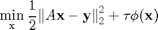
The unconstrained optimization pronblem of regularized image recovery is presented as below:

$\min \limits_{\mathbf{x}} \frac{1}{2}{\left\|A\mathbf{x}-\mathbf{y}\right\|} _2^2 + \tau \phi(\mathbf{x})$

- 2.1 Variable Splitting

Variable splitting is a very simple procedure that consists of creating a new variable, say $v$ , to serve as the argument of ${f_2}(x)$ under the constraint that $g(u) = v$ .

Using variable splitting, we can convert the objective function to the sum of two functions, one of which is written as the composition of two functions:

$\min \limits_{\mathbf{u}\in {\mathcal{R}}^n} {f_1}(\mathbf{u}) + {f_2}(g(\mathbf{u})) $$ , where $$ g : {\mathcal{R}}^n \rightarrow {\mathcal{R}}^d$

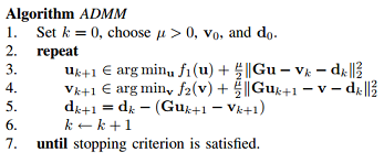
- 2.2 Algorithm ADMM

- 2.3 Optimization Formulation of Image Recovery

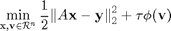
Recall the unconstrained optimization problem of regularized image recovery defined above, we can rewrite this problem in variable splitting form as follows :

${f_1}(\mathbf{x}) = \frac{1}{2}{\left\|A\mathbf{x}-\mathbf{y}\right\|} _2^2$

${f_2}(\mathbf{x}) = \tau \phi(\mathbf{x})$

$\mathbf{G} = \mathbf{I}$

The constrained optimization formulation is thus

$\min \limits_{\mathbf{x}, \mathbf{v} \in {\mathcal{R}}^n} \frac{1}{2}{\left\|A\mathbf{x}-\mathbf{y}\right\|} _2^2 + \tau \phi(\mathbf{v})$

subject to $\mathbf{x} = \mathbf{v}$

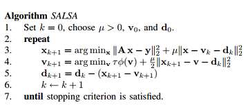
- 2.4 Algorithm SALSA

Inserting the definitions given in above in the ADMM algorithm yields the proposed SALSA (split augmented Lagrangian shrinkage algorithm).

3. Solution and Results

Below is the matlab code and visulization results of the three problems we mentioned in section 1 problem formulation.

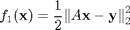
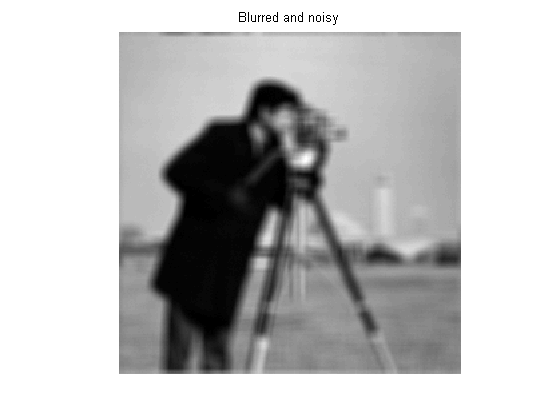
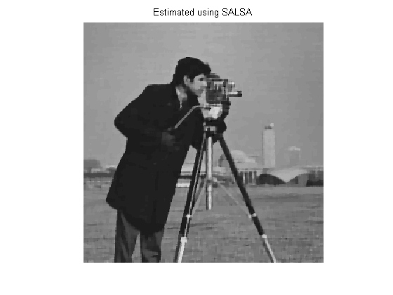
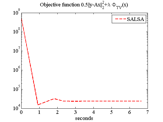
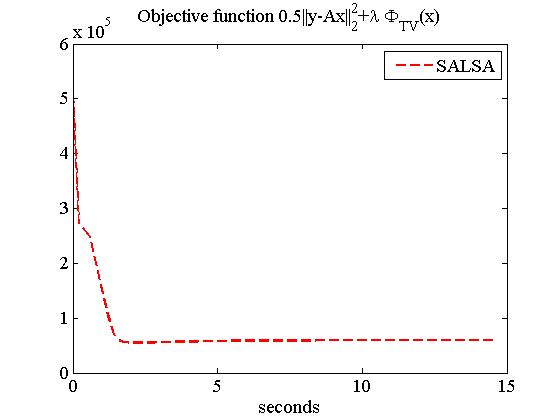
- 3.1 Image Deblurring with Total Variation

%%%%%%%%%%%%%%%%%% *Iamge Debluring with Total Variation %%%%%%%%%%%%%
% Demo of image deblurring, with total variation.
% 9*9 uniform blur, and Gaussian noise (SNR = 40 dB).

close all;
clear;

%%%% original image
x = double( imread('cameraman.tif') );
[M, N] = size(x);

%%%% function handle for uniform blur operator (acts on the image
%%%% coefficients)
h = [1 1 1 1 1 1 1 1 1];
lh = length(h);
h = h/sum(h);
h = [h zeros(1,length(x)-length(h))];
h = cshift(h,-(lh-1)/2);
h = h'*h;

H_FFT = fft2(h);
HC_FFT = conj(H_FFT);

A = @(x) real(ifft2(H_FFT.*fft2(x)));
AT = @(x) real(ifft2(HC_FFT.*fft2(x)));

global calls;
calls = 0;
A = @(x) callcounter(A,x);
AT = @(x) callcounter(AT,x);

%%%%% observation
Ax = A(x);
Psig  = norm(Ax,'fro')^2/(M*N);
BSNRdb = 40;
sigma = norm(Ax-mean(mean(Ax)),'fro')/sqrt(N*M*10^(BSNRdb/10));

y = Ax + sigma*randn(M,N);

%%%% algorithm parameters
lambda = 2.5e-2; % reg parameter
mu = lambda/10;
outeriters = 500;
tol = 1e-5;

%%%% TV regularization
Phi_TV = @(x) TVnorm(x);
chambolleit = 5;
Psi_TV = @(x,th)  mex_vartotale(x,th,'itmax',chambolleit);

filter_FFT = 1./(abs(H_FFT).^2 + mu);
invLS = @(x) real(ifft2(filter_FFT.*fft2( x )));

invLS = @(x) callcounter(invLS,x);

fprintf('Running SALSA...\n')
[x_salsa, numA, numAt, objective, distance, times, mses] = ...
         SALSA_v2(y, A, lambda,...
         'MU', mu, ...
         'AT', AT, ...
         'StopCriterion', 1, ...
         'True_x', x, ...
         'ToleranceA', tol,...
         'MAXITERA', outeriters, ...
         'Psi', Psi_TV, ...
         'Phi', Phi_TV, ...
         'TVINITIALIZATION', 1, ...
         'TViters', 10, ...
         'LS', invLS, ...
         'VERBOSE', 0);
mse = norm(x-x_salsa,'fro')^2 /(M*N);
ISNR = 10*log10( norm(y-x,'fro')^2 / (mse*M*N) );
cpu_time = times(end);

calls_salsa = calls;
calls = 0;

fprintf('SALSA\n CPU time = %3.3g seconds, iters = %d \tMSE = %3.3g, ISNR = %3.3g dB\n', cpu_time, length(objective), mse, ISNR)

figure, imagesc(x), title('original'), colormap gray, axis equal, axis off
title('original')

figure, imagesc(y), colormap gray, axis equal, axis off
title('Blurred and noisy')

figure, imagesc(x_salsa), title('Estimated'), colormap gray, axis equal, axis off;
title('Estimated using SALSA')

figure, semilogy(times, objective,'r--', 'LineWidth',1.8),
title('Objective function 0.5||y-Ax||_{2}^{2}+\lambda \Phi_{TV}(x)','FontName','Times','FontSize',14),
set(gca,'FontName','Times'),
set(gca,'FontSize',14),
xlabel('seconds'),
legend('SALSA');

Running SALSA...
Warning: user specified Phi and Psi will not be used as TV with initialization flag has been set to 1.
SALSA
 CPU time = 6.65 seconds, iters = 36 	MSE = 87.5, ISNR = 7.94 dB

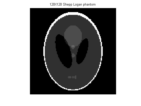
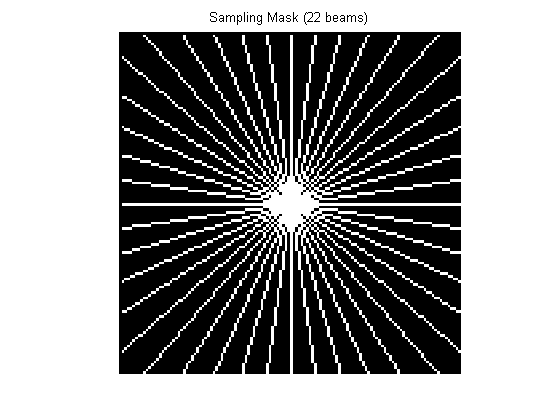
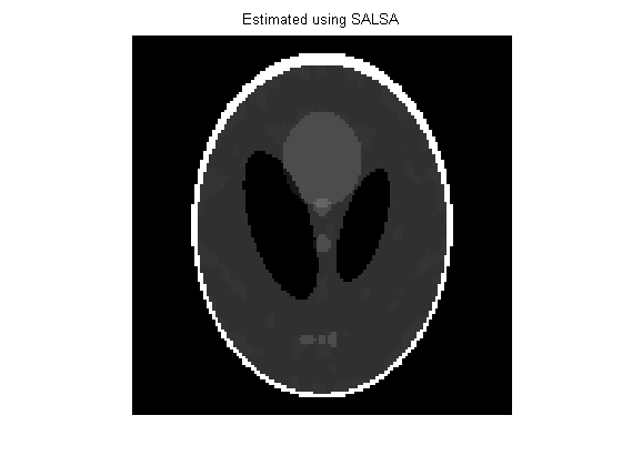
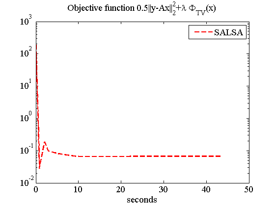
- 3.2 MRI Image Reconstruction

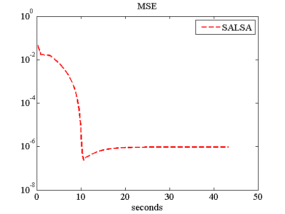
%%%%%%%%%%%%%%%%%% *MRI Image Reconstuction %%%%%%%%%%%%%%%%%%%%%%%%%%
% Demo of MRI image reconstruction, with total variation.
% 128*128 SHepp-Logan phantom, 22 radial lines.

N = 128;
x = phantom(N);
angles = 22;

[mask_temp,Mh,mi,mhi] = LineMask(angles,N);
mask = fftshift(mask_temp);
A = @(x)  masked_FFT(x,mask);
AT = @(x) (masked_FFT_t(x,mask));
ATA = @(x) (ifft2c(mask.*fft2c(x))) ;

global calls;
calls = 0;
A = @(x) callcounter(A,x);
AT = @(x) callcounter(AT,x);
ATA = @(x) callcounter(ATA,x);

sigma =  1e-3/sqrt(2);
y = A(x);
y = y + sigma*(randn(size(y)) + i*randn(size(y)));

%%%% TV regularization
chambolleit = 40;
Psi_TV = @(x,th)  projk(real(x),th,chambolleit);
Phi_TV = @(x) TVnorm(real(x));

%%%% algorithm parameters
lambda = 9e-5;
mu = lambda*100;
inneriters = 5;
outeriters = 1000;
tol = 5e-6;

invLS = @(x) (x - (1/(1+mu))*ATA(x) )/mu;

fprintf('Running SALSA...\n')
[x_salsa, numA, numAt, objective, distance,  times, mses]= ...
         SALSA_v2(y,A,lambda,...
         'AT', AT, ...
         'Mu', mu, ...
         'Psi', Psi_TV, ...
         'Phi', Phi_TV, ...
         'True_x', x,...
         'TVINITIALIZATION', 0, ...
         'StopCriterion', 1,...
       	 'ToleranceA', tol, ...
         'MAXITERA', outeriters, ...
         'LS', invLS, ...
         'Verbose', 0);

mse_salsa = norm(x- x_salsa,'fro')^2/numel(x);
time_salsa = times(end);

calls_salsa = calls;
calls = 0;

fprintf('SALSA:\nIters = %d, calls = %d, CPU time = %g seconds, MSE = %g\n', length(objective), calls_salsa, time_salsa, mse_salsa)

figure, imagesc(x),colormap(gray), axis equal, axis off,
title('128X128 Shepp Logan phantom');

figure, imagesc(mask), colormap gray, axis equal, axis off,
title('Sampling Mask (22 beams)');

figure, imagesc(real(x_salsa)), colormap gray, axis equal, axis off,
title('Estimated using SALSA');

figure, semilogy(times, objective,'r--', 'LineWidth',1.8),
title('Objective function 0.5||y-Ax||_{2}^{2}+\lambda \Phi_{TV}(x)','FontName','Times','FontSize',14),
set(gca,'FontName','Times'),
set(gca,'FontSize',14),
xlabel('seconds'),
legend('SALSA');

figure, semilogy(times, mses,'r--', 'LineWidth',1.8),
title('MSE','FontName','Times','FontSize',14),
set(gca,'FontName','Times'),
set(gca,'FontSize',14),
xlabel('seconds'),
legend('SALSA');

Running SALSA...
SALSA:
Iters = 398, calls = 799, CPU time = 43.3059 seconds, MSE = 9.60275e-07

- 3.3 Image Inpainting

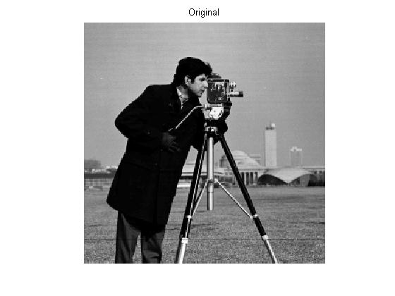
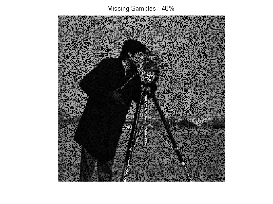
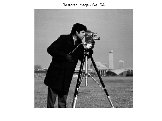
%%%%%%%%%%% *Image Inpainting %%%%%%%%%%%%%%
% Demo of image inpainting (with 40% of the pixels missing), with total variation.

x = double(imread('cameraman.tif'));
N=length(x);

% random observations
O = rand(N)> 0.4;    % 40% missing
y= x.* O;

% set BSNR
BSNR = 40;
Py = var(x(:));
sigma= sqrt((Py/10^(BSNR/10)));
% add noise
y=y+ sigma*randn(N);
y = y.*O;

% handle functions for TwIST
%  convolution operators
A = @(x)  O.*x;
AT = @(x) O.*x;

global calls;
calls = 0;
A = @(x) callcounter(A,x);
AT = @(x) callcounter(AT,x);

% denoising function;
chambolleit = 20;
Psi_TV = @(x,th)  projk(real(x),th,chambolleit);
% TV regularizer;
Phi_TV = @(x) TVnorm(x);

%%%% parameters
lambda = 0.2*sigma^2;
mu = 5e-3;
tolA = 1e-4;
outeriters = 500;

%%%% SALSA

invATA = O*(1/(1+mu))+(1-O)*(1/mu);
invLS = @(x) invATA.*x;
invLS = @(x) callcounter(invLS,x);

%%%% SALSA
fprintf('Running SALSA...\n')
[x_salsa, numA, numAt, objective, distance,  times, mses]= ...
         SALSA_v2(y,A,lambda,...
         'MU', mu, ...
         'AT', AT, ...
         'True_x', x,...
         'TVINITIALIZATION', 0, ...
         'Psi', Psi_TV, ...
         'Phi', Phi_TV, ...
         'StopCriterion', 1,...
       	 'ToleranceA', tolA,...
         'Initialization',y,...
         'MAXITERA', outeriters, ...
         'LS', invLS, ...
         'Verbose', 0);

mse_salsa = norm(x- x_salsa,'fro')^2/numel(x);
ISNR_salsa = 10*log10( sum((y(:)-x(:)).^2)./(mse_salsa*numel(x)) );
time_salsa = times(end);

calls_salsa = calls;
calls = 0;

fprintf('SALSA\nCPU time = %3.3g seconds, calls = %d \titers = %d \tMSE = %3.3g, ISNR = %3.3g dB\n', time_salsa, calls_salsa, length(objective), mse_salsa, ISNR_salsa)

figure, colormap(gray), imagesc(x), axis equal, axis off, title('Original');

figure, colormap gray, imagesc(y), axis equal, axis off, title('Missing Samples - 40%');

figure, imagesc(x_salsa), colormap gray, axis equal, axis off, title('Restored Image - SALSA');

figure, plot(times, objective,'r--', 'LineWidth',1.8),
title('Objective function 0.5||y-Ax||_{2}^{2}+\lambda \Phi_{TV}(x)','FontName','Times','FontSize',14),
set(gca,'FontName','Times'),
set(gca,'FontSize',14),
xlabel('seconds'),
legend('SALSA');

Running SALSA...
SALSA
CPU time = 14.5 seconds, calls = 148 	iters = 73 	MSE = 88.3, ISNR = 19.1 dB

Analysis and Conclusion

In this project, we reproduced the results for the unconstrained optimization formulation of regularized image reconstruction / restoration using the SALSA. This approach is based on a variable splitting technique which yields an equivalent constrained problem. Then this constrained problem is then addressed using ADMM. Therefore, this is SALSA that presented in [1].

For all experiments, we used total variation for regularization. In total we did three standard image recovery problems (deconvolution, MRI reconstruction, inpainting) using the proposed algorithm (SALSA, for split augmented Lagrangian shrinkage algorithm).

Furthermore, we observed that we achieved a smaller running time than presented in the paper. The reason is that the running environment is improved compared with the running environment in the paper. For all three experiments we conducted using MATLAB, on a computer equipped with an Intel® Core™ i5-3330 3.00 GHz processor, with 8.00 GB of RAM and running Windows 7 Enterprise.

The results obtained are consistent with the paper. From redsults we can see that this algorithm has a good performance including image recovery output and running time.

Refenrences and Links

[1] Afonso, Manya V., José M. Bioucas-Dias, and Mário AT Figueiredo. "Fast image recovery using variable splitting and constrained optimization." IEEE Transactions on Image Processing 19.9 (2010): 2345-2356.

[2] http://cascais.lx.it.pt/~mafonso/salsa.html