Contents
- 1. Introduction
- 2. Problem Formulation
- 3. Proposed Solution
- 4. Generating a Random Network, As Stated in the Paper, and Showing Its Toplogy
- 5. Finding Parameters of the Randomly Generated Network and Setting Up the Links Between the Nodes
- 6. Simultaneous Optimization of the Routing and Resource Allocation
- 7. Plotting the Optimal Routing, Aggregate Flow in the Network, and Optimal Power Allocation over the Links (for the case of simultaneous optimization)
- 7.1. Plotting the ptimal data routing for the source_dest_nodes(1),(results corresponding to Fig.2(a) in the paper):
- 7.2. Plotting the ptimal data routing for the source_dest_nodes(2), (results corresponding to Fig.2(b) in the paper):
- 7.3. Plotting aggregate flow for all destinations(results corresponding to Fig.2(c) in the paper):
- 7.4. Plotting optimal power allocation over the links across the network (results corresponding to Fig.2(d) in the paper):
- 8. Disjoint Optimization of the Routing and Resource Allocation and Comparing with Joint Optimization
- 9. Analysis and Conclusions
- 10. References
%%%%%%%%%%%%%%%%%%%%%%%%%%%%%%%%%%%%%%%%%%%%%%%%%%%%%%
% ECE 602, Intro to Optimization, Course Final Project
% Saber Malekmohammadi, 20691166
% University of Waterloo,Winter 2017
%%%%%%%%%%%%%%%%%%%%%%%%%%%%%%%%%%%%%%%%%%%%%%%%%%%%%%
1. Introduction
As the demand for wireless communication increases, efficient usage of radio resources grows in importance. In traditional routing problems in data networks, the problem has been often formulated as a convex multicommodity network flow problem. In these problems, the capacities of the links, are determined by the allocation of communication resources(such as transmit power and bandwidth) to the links. The optimal performance of the network can only be achieved by the "simultaneous" optimization of routing and resource allocation. In this paper, a method for "joint" optimization of the routing in the network layer and the resource allocation in the physical layer is proposed.
2. Problem Formulation
The authors have used the standard directed graph model to represent the network topology, and a multicommodity flow model for the average behaviour of the data transmissions across the network. For representing the topology of the network and modeling the network layer, the node-link incidence matrix model has been used. A multicommodity flow model for the routing of the data packets across the network has been used. Flows with the same destintion are considered as one single commodity, regardless of their sources. We assume that the destination nodes are labeled d= 1,...,5 . For each destination d, we define a source sink vector s_d which is in R^5 whose n-th entry denotes the nonnegative amount of flow injected in the network at node n destined to the node d. Corresponding to this destination node, we define a flow vector x_d, in R^L, whose l-th entry denotes the nonnegative amount of flow in the l-th link of the network destined to the destination d. Therefore for each of the links in the network, we can define a total flow which is equal to the sum of {x_d(i)}s for d=1,...,5. We denote this total flow in the i-th link by t_i. Also we denote the capacity of this link by C_i. Therefore routing in the "network layer" can be modeled by the following groups of constraints:
% A*x_d = s_d
% x_d >= 0 and s_d >= 0
% d=1,...,5

% for i=1,...,L: t_i  = sum(x_d(i)) over d=1,...,5


% The communication resource constraints can also be modeled. We will use the following model to relate the vector of total traffic and the vector of communcation
% resources that are to be distributed in the network:

% t_i <= c_i , i= 1,...,L
% F*r <= g

% where r is the vector of communication resources allocated to each link and g is the vector of total resources that each node has and is going to distribute
% it among its outgoing links.
3. Proposed Solution
The method that the authors have provided is focused on "joint" optimization of routing in the network layer and resource allocation in the physical layer of the network. We know that the optimal routing of data in the network depends on the link capacities. In traditinal routing optimization problems, these link capacities are usually assumed to be fixed. In wireless communication link capacities are not necessarily fixed, but can be adjusted by the allocation of the communication resources, such as transmit powers, bandwidths, to different links. In this paper, the authors have studied the simultaneous routing and resource allocation (SRRA) problem for wireless data networks within a convex optimization framework: We can combine the flow model of the network layer mentioned above and the link capacity constraints and get a model for whole the network. This model reflects how the link capacities depend on the allocation of the communication resources and how the overall optimal performance of the network can only be achieved by "simultaneous" optimiation of routing and resource allocation. Suppose that the objective is to maximize a concave cost function f(x,s,t,c). The formulation of the problem, considering the constraints that we mentioned above, is:
% max f(x,s,t,c)
% s.t.

% A*x_d = s_d
% x_d >= 0 and s_d >= 0
% for d=1,...,5

% for i=1,...,L: t_i  = sum(x_d(i)) over d=1,...,5


% t_i <= c_i , i= 1,...,L
% F*r <= g ,


% Here in our simulation, the objective functon "f" is sum(log(s_d(i))) over d = 1,...,5 and i= 1,...,5 and i ~= d. Actually, we consider a logarithmic utility
% function  for the network and are going to maximize it by "joint" optimization of routing in network layer and resource allocation in physical layer. We expect
% that by going from disjoint optimization of the two layers in network stack to joint optimization of them (SRRA), this network utility function increase.
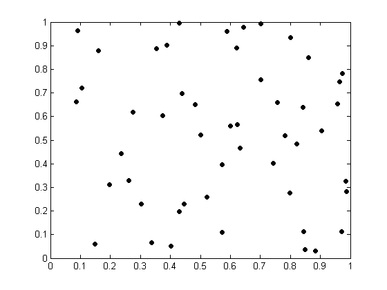
4. Generating a Random Network, As Stated in the Paper, and Showing Its Toplogy
% To demonstrate te benefits of SRRA, we consider a wireless network that is randomly generated by drawing 50 node positions from a unit distribution
% on the unit square [0,1]*[0,1].
    nodes_coordinates = rand (50,2);


% Now we plot the topology of the randomly generated wireless network with 50 nodes:
    figure();
    plot(nodes_coordinates(:,1),nodes_coordinates(:,2),'bO','linewidth',0.5,...
    'markeredgecolor','k','markerfacecolor','k','markersize',5);
5. Finding Parameters of the Randomly Generated Network and Setting Up the Links Between the Nodes
% As stated in the paper, we allow two nodes to communicate if their distance is smaller than the threshold 0.25 (so some of the nodes, which are far, may
% have no connections to other nodes). We then store the information of these connections in a matrix "nodes_conncetions_matrix" :
    nodes_connections_matrix = zeros(50,50);
    k=0;
    for i=1:49
        for j=i+1:50
           if norm (nodes_coordinates(i,:)-nodes_coordinates(j,:))<0.25
            nodes_connections_matrix(i,j)  =  1;
            nodes_connections_matrix(j,i)  =  1;
           end
        end
    end


% Here we make a coloumn vector that its i-th element shows the number of outgoing links from i-th node:
    nodes_outgoing_edges_number = (sum(nodes_connections_matrix'))';


% The total number of links in the network:
    L = sum(nodes_outgoing_edges_number);


% Now using the "nodes_connections_matrix" that we made above, we find origin and destination of every link existing in the network and store this
% information in a matrix "links_origin_dest_info":
    links_origin_dest_info = zeros (L,2);
    k=1;
    for i=1:50
        for j=1:50
            if nodes_connections_matrix(i,j)  ==  1
               links_origin_dest_info(k,:)    =   [i,j];
               k=k+1;
            end
        end
    end


% Now that we have found the information of origin and destination of the links in the network, we can use it to find the "node_link incidence matrix", (A),
% of the network:

    A = zeros(50,L); % node-edge incidence matrix

    for i=1:L
        A((links_origin_dest_info(i,1)),i) =  1;
        A((links_origin_dest_info(i,2)),i) = -1;
    end


% Now we trace all the links existing in the network and plot them:
    for i=1:L
        origin           =  [  nodes_coordinates(links_origin_dest_info(i,1),1)  ,   nodes_coordinates(links_origin_dest_info(i,1),2)   ];
        destination      =  [  nodes_coordinates(links_origin_dest_info(i,2),1)  ,   nodes_coordinates(links_origin_dest_info(i,2),2)   ];

        x_components     =  [  nodes_coordinates(links_origin_dest_info(i,1),1)  ,   nodes_coordinates(links_origin_dest_info(i,2),1)   ];
        [min_x,argmin_x] =     min (x_components);
        [max_x,argmax_x] =     max (x_components);


        x_edge =  min_x + linspace(0,abs (nodes_coordinates(links_origin_dest_info(i,1),1)  -  nodes_coordinates(links_origin_dest_info(i,2),1)) , 100);
        y_edge =  nodes_coordinates(links_origin_dest_info(i,argmin_x),2) + linspace (0,     ( nodes_coordinates(links_origin_dest_info(i,argmax_x),2)-...
                  nodes_coordinates(links_origin_dest_info(i,argmin_x),2) ),100);

        hold on
        plot( x_edge , y_edge );
    end


% Now we choose randomly 5 source and destination nodes S1,S2,S3,S4,S5 and mark them with 5 red markers in the toplogy of the network. Other (50-5) nodes
% will act as relay nodes in the network:

    source_dest_nodes = randsample(50,5); % this 5*1 vector contains the number of those nodes in the network that are not only a relay node. They are sources
                                          % and destinations of the flows which are to be carried over the network.
    hold on
    plot(nodes_coordinates(source_dest_nodes(1),1),nodes_coordinates(source_dest_nodes(1),2),'bO','linewidth',0.5,'markeredgecolor','r',...
        'markerfacecolor','r','markersize',12);

    hold on
    plot(nodes_coordinates(source_dest_nodes(2),1),nodes_coordinates(source_dest_nodes(2),2),'bO','linewidth',0.5,'markeredgecolor','r',...
        'markerfacecolor','r','markersize',12);

    hold on
    plot(nodes_coordinates(source_dest_nodes(3),1),nodes_coordinates(source_dest_nodes(3),2),'bO','linewidth',0.5,'markeredgecolor','r',...
        'markerfacecolor','r','markersize',12);

    hold on
    plot(nodes_coordinates(source_dest_nodes(4),1),nodes_coordinates(source_dest_nodes(4),2),'bO','linewidth',0.5,'markeredgecolor','r',...
        'markerfacecolor','r','markersize',12);

    hold on
    plot(nodes_coordinates(source_dest_nodes(5),1),nodes_coordinates(source_dest_nodes(5),2),'bO','linewidth',0.5,'markeredgecolor','r',...
        'markerfacecolor','r','markersize',12);
     title('topology of the network (red markers are "source and dest" nodes)')


% The gaussin noise powers at the receivers, and at the end of each one of the links, are generated randomly, with a uniform distribution on the interval [0.01,0.1]:
    links_noise_variances = 0.01 + (0.1-0.01) .* rand(L,1);


% Now we find the links lengths to use them for finding each link capacity:
% let Y be the vector containing the distances between the two end nodes of the links in the network:
    Y = zeros (L,1);
     for i=1:L
        Y(i) = norm( nodes_coordinates(links_origin_dest_info(i,1),:) - nodes_coordinates(links_origin_dest_info(i,2),:)   );
     end
    path_loss = (min(Y)./Y).^2;

6. Simultaneous Optimization of the Routing and Resource Allocation
% We define 5 network flow vectors each one corresponding to one of the 5 nodes in "source_dest_nodes" being as destination of flows. Also we apply their
% constraints to be nonnegative
    cvx_begin
    variables x_1(L,1) x_2(L,1) x_3(L,1) x_4(L,1) x_5(L,1)
    x_1 >= 0
    x_2 >= 0
    x_3 >= 0
    x_4 >= 0
    x_5 >= 0


% For each node in "source_dest_nodes" (totally five nodes), we define a source-vector s_i in R^5 which contains the flow input from each one of the
% 5 nodes to the network. Flow input from the other (50-5) nodes are zero, because they were considered to be as relay nodes.
  variables s_1(5,1) s_2(5,1) s_3(5,1) s_4(5,1) s_5(5,1)

  s_1(2)>=0
  s_1(3)>=0
  s_1(4)>=0
  s_1(5)>=0
  s_1(1)== -(s_1(2)+s_1(3)+s_1(4)+s_1(5))% in order for the flows destined to the first node in "source_dest_nodes" to be balanced.

  s_2(1)>=0
  s_2(3)>=0
  s_2(4)>=0
  s_2(5)>=0
  s_2(2)== -(s_2(1)+s_2(3)+s_2(4)+s_2(5))% in order for the flows destined to the second node in "source_dest_nodes" to be balanced.

  s_3(1)>=0
  s_3(2)>=0
  s_3(4)>=0
  s_3(5)>=0
  s_3(3)== -(s_3(1)+s_3(2)+s_3(4)+s_3(5))% in order for the flows destined to the third node in "source_dest_nodes" to be balanced.

  s_4(1)>=0
  s_4(2)>=0
  s_4(3)>=0
  s_4(5)>=0
  s_4(4)== -(s_4(1)+s_4(2)+s_4(3)+s_4(5))% in order for the flows destined to the fourth node in "source_dest_nodes" to be balanced.

  s_5(1)>=0
  s_5(2)>=0
  s_5(3)>=0
  s_5(4)>=0
  s_5(5)== -(s_5(1)+s_5(2)+s_5(3)+s_5(4))% in order for the flows destined to the fifth node in "source_dest_nodes" to be balanced.


% Imposing the constraints of flow conservations (Ax=b) in the network for each one of the five source_destination flows :
    for i= 1:50
      if i == source_dest_nodes(1)
         A(i,:)*x_1 == s_1(1)
         A(i,:)*x_2 == s_2(1)
         A(i,:)*x_3 == s_3(1)
         A(i,:)*x_4 == s_4(1)
         A(i,:)*x_5 == s_5(1)

          else if i == source_dest_nodes(2)
                  A(i,:)*x_1 == s_1(2)
                  A(i,:)*x_2 == s_2(2)
                  A(i,:)*x_3 == s_3(2)
                  A(i,:)*x_4 == s_4(2)
                  A(i,:)*x_5 == s_5(2)

                    else if i == source_dest_nodes(3)
                            A(i,:)*x_1 == s_1(3)
                            A(i,:)*x_2 == s_2(3)
                            A(i,:)*x_3 == s_3(3)
                            A(i,:)*x_4 == s_4(3)
                            A(i,:)*x_5 == s_5(3)

                              else if i == source_dest_nodes(4)
                                      A(i,:)*x_1 == s_1(4)
                                      A(i,:)*x_2 == s_2(4)
                                      A(i,:)*x_3 == s_3(4)
                                      A(i,:)*x_4 == s_4(4)
                                      A(i,:)*x_5 == s_5(4)

                                        else if i == source_dest_nodes(5)
                                                A(i,:)*x_1 == s_1(5)
                                                A(i,:)*x_2 == s_2(5)
                                                A(i,:)*x_3 == s_3(5)
                                                A(i,:)*x_4 == s_4(5)
                                                A(i,:)*x_5 == s_5(5)

                                                  else

                                                   A(i,:)*x_1 == 0
                                                   A(i,:)*x_2 == 0
                                                   A(i,:)*x_3 == 0
                                                   A(i,:)*x_4 == 0
                                                   A(i,:)*x_5 == 0
                                            end
                                  end
                        end
          end


    end
end


% We are free to adjust the transmit powers Pl allocated to each link (Resource Allocation). So we define a vector L*1 of variables, the powers of the L
% links in the network:

    variables links_power(L,1)
    links_power >= 0 % applying the constraint on them to be nonnegative


% We should impose a total power constraint for the outgoing links of each node, which has a total power budget equal to 100:
    p_tot = 100*ones(50,1);
    A_plus = floor((A+1)/2); % A matrix which has the same size as the incidence matrix A, and its elements are given
                             % by A_plus(n,l) = max{0 , A(n,l)}, which only
                             % identify the outgoing links at each node.
    A_plus*links_power <= p_tot


% The power at the receiver at the end of i-th link is given by (path_loss(i) * links_power(i)). Also th eadditive noise power at the end of this link is
% equal to links_noise_variances(i). We link the capacity formula with unit bandwidth : log (1+(path_loss(i)*(links_power(i)/links_noise_variances(i))))
% So the capacity constraint on each of the links of the network should be imposed:
    for i=1:L
        x_1(i)+x_2(i)+x_3(i)+x_4(i)+x_5(i) <= log (1+(path_loss(i)*(links_power(i)/links_noise_variances(i))))
    end


% We consider the problem of joint optimization of routing and power allocation to maximize the totality of the network, where all (source,destination)
% pairs (chosen from the five nodes in "source_dest_nodes") have the logarithmic utility function: log (flow)

    maximize (log(s_1(2))+log(s_1(3))+log(s_1(4))+log(s_1(5))+log(s_2(1))+log(s_2(3))+...
              log(s_2(4))+log(s_2(5))+log(s_3(1))+log(s_3(2))+log(s_3(4))+log(s_3(5))+...
              log(s_4(1))+log(s_4(2))+log(s_4(3))+log(s_4(5))+log(s_5(1))+log(s_5(2))+...
              log(s_5(3))+log(s_5(4)));
    cvx_end

% Storing the obtained maximum network utility in a variable:

    max_utility_1 = log(s_1(2))+log(s_1(3))+log(s_1(4))+log(s_1(5))+log(s_2(1))+log(s_2(3))+...
                  log(s_2(4))+log(s_2(5))+log(s_3(1))+log(s_3(2))+log(s_3(4))+log(s_3(5))+...
                  log(s_4(1))+log(s_4(2))+log(s_4(3))+log(s_4(5))+log(s_5(1))+log(s_5(2))+...
                  log(s_5(3))+log(s_5(4)) ;


% Network maximum utility:
    display(sprintf('Network maximum utility, in joint optimization case, is equal to:\n %s \n\n',max_utility_1 ))


% The source and sink flows which achieve the maximum utility:
    display(sprintf('The table below shows the source and sink flows which achieve the maximum total utility of %s.\nThe diagonals are the negative total flows (sinks) destined to one of the five destinations', max_utility_1))
    [s_1,s_2,s_3,s_4,s_5]
Successive approximation method to be employed.
   SDPT3 will be called several times to refine the solution.
   Original size: 3280 variables, 1390 equality constraints
   370 exponentials add 2960 variables, 1850 equality constraints
-----------------------------------------------------------------
 Cones  |             Errors              |
Mov/Act | Centering  Exp cone   Poly cone | Status
--------+---------------------------------+---------
115/115 | 6.145e+00  2.051e+00  0.000e+00 | Solved
 98/ 98 | 1.485e+00  1.424e-01  1.708e-10 | Solved
 96/ 97 | 1.217e-01  9.242e-04  0.000e+00 | Solved
 86/ 96 | 1.765e-02  1.950e-05  0.000e+00 | Solved
 25/ 79 | 2.454e-03  3.768e-07  0.000e+00 | Solved
  0/ 49 | 3.458e-04  7.650e-09  2.101e-10 | Solved
-----------------------------------------------------------------
Status: Solved
Optimal value (cvx_optval): +20.5314

Network maximum utility, in joint optimization case, is equal to:
 2.053137e+01


The table below shows the source and sink flows which achieve the maximum total utility of 2.053137e+01.
The diagonals are the negative total flows (sinks) destined to one of the five destinations

ans =

   -5.9919    2.2230    2.1258    1.4209    1.4209
    1.7850  -17.3403    6.8714    3.4129    3.4129
    1.6411    7.3265  -15.1302    2.5613    2.5613
    1.2411    3.5136    2.8290  -14.0668    4.9826
    1.3246    4.2772    3.3039    6.6717  -12.3777
7. Plotting the Optimal Routing, Aggregate Flow in the Network, and Optimal Power Allocation over the Links (for the case of simultaneous optimization)
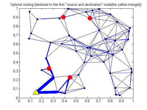
7.1. Plotting the ptimal data routing for the source_dest_nodes(1),(results corresponding to Fig.2(a) in the paper):
figure();plot(nodes_coordinates(:,1),nodes_coordinates(:,2),'bO','linewidth',0.5,'markeredgecolor','k','markerfacecolor','k','markersize',5);
for i=1:L


    if x_1(i)> 0.0001

            origin           =  [  nodes_coordinates(links_origin_dest_info(i,1),1)  ,   nodes_coordinates(links_origin_dest_info(i,1),2)   ];
            destination      =  [  nodes_coordinates(links_origin_dest_info(i,2),1)  ,   nodes_coordinates(links_origin_dest_info(i,2),2)   ];

            x_components     =  [  nodes_coordinates(links_origin_dest_info(i,1),1)  ,   nodes_coordinates(links_origin_dest_info(i,2),1)   ];
            [min_x,argmin_x] =     min (x_components);
            [max_x,argmax_x] =     max (x_components);


           x_edge =  min_x + linspace(0,abs  (nodes_coordinates(links_origin_dest_info(i,1),1)  -  nodes_coordinates(links_origin_dest_info(i,2),1)) , 100);
           y_edge =  nodes_coordinates(links_origin_dest_info(i,argmin_x),2) + linspace (0,  ( nodes_coordinates(links_origin_dest_info(i,argmax_x),2)-...
               nodes_coordinates(links_origin_dest_info(i,argmin_x),2) ),100);

           hold on
           plot( x_edge , y_edge , 'linewidth', 25* x_1(i)/log(10000));
    end

end

hold on
plot(nodes_coordinates(source_dest_nodes(1),1),nodes_coordinates(source_dest_nodes(1),2),'b^','linewidth',0.5,'markeredgecolor','k',...
    'markerfacecolor','y','markersize',15);

hold on
plot(nodes_coordinates(source_dest_nodes(2),1),nodes_coordinates(source_dest_nodes(2),2),'bO','linewidth',0.5,'markeredgecolor','r',...
    'markerfacecolor','r','markersize',12);

hold on
plot(nodes_coordinates(source_dest_nodes(3),1),nodes_coordinates(source_dest_nodes(3),2),'bO','linewidth',0.5,'markeredgecolor','r',...
    'markerfacecolor','r','markersize',12);

hold on
plot(nodes_coordinates(source_dest_nodes(4),1),nodes_coordinates(source_dest_nodes(4),2),'bO','linewidth',0.5,'markeredgecolor','r',...
'markerfacecolor','r','markersize',12);

hold on
plot(nodes_coordinates(source_dest_nodes(5),1),nodes_coordinates(source_dest_nodes(5),2),'bO','linewidth',0.5,'markeredgecolor','r',...
    'markerfacecolor','r','markersize',12);
title('Optimal routing (destined to the first "source and destination" node(the yellow triangle))')
7.2. Plotting the ptimal data routing for the source_dest_nodes(2), (results corresponding to Fig.2(b) in the paper):
figure();plot(nodes_coordinates(:,1),nodes_coordinates(:,2),'bO','linewidth',0.5,'markeredgecolor','k','markerfacecolor','k','markersize',5);
for i=1:L


    if x_2(i)> 0.0001

            origin           =  [  nodes_coordinates(links_origin_dest_info(i,1),1)  ,   nodes_coordinates(links_origin_dest_info(i,1),2)   ];
            destination      =  [  nodes_coordinates(links_origin_dest_info(i,2),1)  ,   nodes_coordinates(links_origin_dest_info(i,2),2)   ];

            x_components     =  [  nodes_coordinates(links_origin_dest_info(i,1),1)  ,   nodes_coordinates(links_origin_dest_info(i,2),1)   ];
            [min_x,argmin_x] =     min (x_components);
            [max_x,argmax_x] =     max (x_components);


            x_edge =  min_x + linspace(0,abs  (nodes_coordinates(links_origin_dest_info(i,1),1)  -  nodes_coordinates(links_origin_dest_info(i,2),1)) , 100);
            y_edge =  nodes_coordinates(links_origin_dest_info(i,argmin_x),2) + linspace (0,  ( nodes_coordinates(links_origin_dest_info(i,argmax_x),2)-...
                     nodes_coordinates(links_origin_dest_info(i,argmin_x),2) ),100);

            hold on
            plot( x_edge , y_edge , 'linewidth', 25* x_2(i)/log(10000));
    end

end

hold on
plot(nodes_coordinates(source_dest_nodes(1),1),nodes_coordinates(source_dest_nodes(1),2),'bO','linewidth',0.5,'markeredgecolor','k',...
    'markerfacecolor','r','markersize',12);

hold on
plot(nodes_coordinates(source_dest_nodes(2),1),nodes_coordinates(source_dest_nodes(2),2),'b^','linewidth',0.5,'markeredgecolor','r',...
    'markerfacecolor','y','markersize',15);

hold on
plot(nodes_coordinates(source_dest_nodes(3),1),nodes_coordinates(source_dest_nodes(3),2),'bO','linewidth',0.5,'markeredgecolor','r',...
    'markerfacecolor','r','markersize',12);

hold on
plot(nodes_coordinates(source_dest_nodes(4),1),nodes_coordinates(source_dest_nodes(4),2),'bO','linewidth',0.5,'markeredgecolor','r',...
    'markerfacecolor','r','markersize',12);

hold on
plot(nodes_coordinates(source_dest_nodes(5),1),nodes_coordinates(source_dest_nodes(5),2),'bO','linewidth',0.5,'markeredgecolor','r',...
    'markerfacecolor','r','markersize',12);
title('Optimal routing (to the second "source and destination" node (the yellow triangle)')

% Optimal routing to other destination nodes are omitted since they have similar patterns.

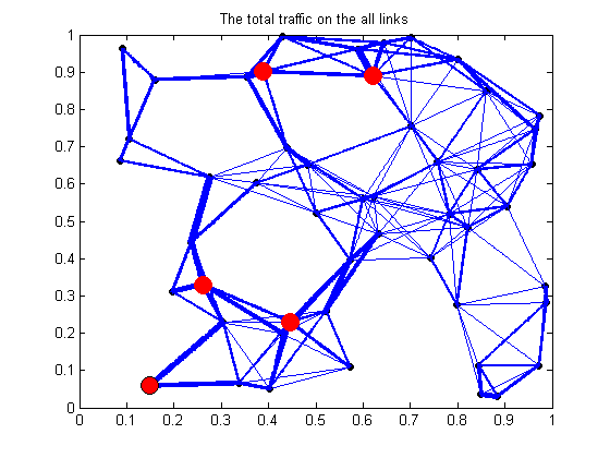
7.3. Plotting aggregate flow for all destinations(results corresponding to Fig.2(c) in the paper):
figure();plot(nodes_coordinates(:,1),nodes_coordinates(:,2),'bO','linewidth',0.5,'markeredgecolor','k','markerfacecolor','k','markersize',5);
for i=1:L


    if x_1(i)+x_2(i)+x_3(i)+x_4(i)+x_5(i)> 0

            origin           =  [  nodes_coordinates(links_origin_dest_info(i,1),1)  ,   nodes_coordinates(links_origin_dest_info(i,1),2)   ];
            destination      =  [  nodes_coordinates(links_origin_dest_info(i,2),1)  ,   nodes_coordinates(links_origin_dest_info(i,2),2)   ];

            x_components     =  [  nodes_coordinates(links_origin_dest_info(i,1),1),     nodes_coordinates(links_origin_dest_info(i,2),1)   ];
            [min_x,argmin_x] =     min (x_components);
            [max_x,argmax_x] =     max (x_components);


           x_edge =  min_x + linspace(0,abs  (nodes_coordinates(links_origin_dest_info(i,1),1)  -  nodes_coordinates(links_origin_dest_info(i,2),1)) , 100);
           y_edge =  nodes_coordinates(links_origin_dest_info(i,argmin_x),2) + linspace (0,    (nodes_coordinates(links_origin_dest_info(i,argmax_x),2)-...
                     nodes_coordinates(links_origin_dest_info(i,argmin_x),2) ),100);

           hold on
           plot( x_edge , y_edge , 'linewidth', ( 10*(x_1(i)+x_2(i)+x_3(i)+x_4(i)+x_5(i)) )/log(10000));
    end

end

hold on
plot(nodes_coordinates(source_dest_nodes(1),1),nodes_coordinates(source_dest_nodes(1),2),'bO','linewidth',0.5,'markeredgecolor','k',...
    'markerfacecolor','r','markersize',12);

hold on
plot(nodes_coordinates(source_dest_nodes(2),1),nodes_coordinates(source_dest_nodes(2),2),'bO','linewidth',0.5,'markeredgecolor','r',...
    'markerfacecolor','r','markersize',12);

hold on
plot(nodes_coordinates(source_dest_nodes(3),1),nodes_coordinates(source_dest_nodes(3),2),'bO','linewidth',0.5,'markeredgecolor','r',...
    'markerfacecolor','r','markersize',12);

hold on
plot(nodes_coordinates(source_dest_nodes(4),1),nodes_coordinates(source_dest_nodes(4),2),'bO','linewidth',0.5,'markeredgecolor','r',...
    'markerfacecolor','r','markersize',12);

hold on
plot(nodes_coordinates(source_dest_nodes(5),1),nodes_coordinates(source_dest_nodes(5),2),'bO','linewidth',0.5,'markeredgecolor','r',...
    'markerfacecolor','r','markersize',12);
title('The total traffic on the all links')
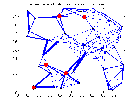
7.4. Plotting optimal power allocation over the links across the network (results corresponding to Fig.2(d) in the paper):
figure();plot(nodes_coordinates(:,1),nodes_coordinates(:,2),'bO','linewidth',0.5,'markeredgecolor','k','markerfacecolor','k','markersize',5);
for i=1:L


    if links_power(i)> 0.001

            origin           =  [  nodes_coordinates(links_origin_dest_info(i,1),1)  ,   nodes_coordinates(links_origin_dest_info(i,1),2)   ];
            destination      =  [  nodes_coordinates(links_origin_dest_info(i,2),1)  ,   nodes_coordinates(links_origin_dest_info(i,2),2)   ];

            x_components     =  [  nodes_coordinates(links_origin_dest_info(i,1),1),     nodes_coordinates(links_origin_dest_info(i,2),1)   ];
            [min_x,argmin_x] =     min (x_components);
            [max_x,argmax_x] =     max (x_components);


           x_edge =  min_x + linspace(0,abs  (nodes_coordinates(links_origin_dest_info(i,1),1)  -  nodes_coordinates(links_origin_dest_info(i,2),1)) , 100);
           y_edge =  nodes_coordinates(links_origin_dest_info(i,argmin_x),2) + linspace (0,  ( nodes_coordinates(links_origin_dest_info(i,argmax_x),2)-...
                     nodes_coordinates(links_origin_dest_info(i,argmin_x),2) ),100);

           hold on
           plot( x_edge , y_edge , 'linewidth', ( 8*links_power(i) )/100);
    end

end

hold on
plot(nodes_coordinates(source_dest_nodes(1),1),nodes_coordinates(source_dest_nodes(1),2),'bO','linewidth',0.5,'markeredgecolor','k',...
    'markerfacecolor','r','markersize',12);

hold on
plot(nodes_coordinates(source_dest_nodes(2),1),nodes_coordinates(source_dest_nodes(2),2),'bO','linewidth',0.5,'markeredgecolor','r',...
    'markerfacecolor','r','markersize',12);

hold on
plot(nodes_coordinates(source_dest_nodes(3),1),nodes_coordinates(source_dest_nodes(3),2),'bO','linewidth',0.5,'markeredgecolor','r',...
'markerfacecolor','r','markersize',12);

hold on
plot(nodes_coordinates(source_dest_nodes(4),1),nodes_coordinates(source_dest_nodes(4),2),'bO','linewidth',0.5,'markeredgecolor','r',...
    'markerfacecolor','r','markersize',12);

hold on
plot(nodes_coordinates(source_dest_nodes(5),1),nodes_coordinates(source_dest_nodes(5),2),'bO','linewidth',0.5,'markeredgecolor','r',...
    'markerfacecolor','r','markersize',12);
title('optimal power allocation over the links across the network')
8. Disjoint Optimization of the Routing and Resource Allocation and Comparing with Joint Optimization
% Now we are going to find the optimal routing if the power has already allocated evenly to the links. i.e., disjoint optimizaion of the routing in the
% network layer and resource allocation in the physical layer. We expect this case not to have a total optimum utility better than that of the simlutaneous
% optimization case:

  cvx_begin


% We define 5 network flow vectors each one corresponding to one of the 5 nodes in "source_dest_nodes" being as destination of flows. Also we apply their constraints to be nonnegative
  variables x_1(L,1) x_2(L,1) x_3(L,1) x_4(L,1) x_5(L,1)
  x_1 >= 0
  x_2 >= 0
  x_3 >= 0
  x_4 >= 0
  x_5 >= 0


% For each node in "source_dest_nodes" (totally five nodes), we define a source-vector s_i in R^5 which contains the flow input from each one of the 5
% nodes to the network. Flow input from the other (50-5) nodes are zero, because they were considered to be as relay nodes.
  variables s_1(5,1) s_2(5,1) s_3(5,1) s_4(5,1) s_5(5,1)

  s_1(2)>=0
  s_1(3)>=0
  s_1(4)>=0
  s_1(5)>=0
  s_1(1)== -(s_1(2)+s_1(3)+s_1(4)+s_1(5))% in order for the flows destined to the first node in "source_dest_nodes" to be balanced.

  s_2(1)>=0
  s_2(3)>=0
  s_2(4)>=0
  s_2(5)>=0
  s_2(2)== -(s_2(1)+s_2(3)+s_2(4)+s_2(5))% in order for the flows destined to the second node in "source_dest_nodes" to be balanced.

  s_3(1)>=0
  s_3(2)>=0
  s_3(4)>=0
  s_3(5)>=0
  s_3(3)== -(s_3(1)+s_3(2)+s_3(4)+s_3(5))% in order for the flows destined to the third node in "source_dest_nodes" to be balanced.

  s_4(1)>=0
  s_4(2)>=0
  s_4(3)>=0
  s_4(5)>=0
  s_4(4)== -(s_4(1)+s_4(2)+s_4(3)+s_4(5))% in order for the flows destined to the fourth node in "source_dest_nodes" to be balanced.

  s_5(1)>=0
  s_5(2)>=0
  s_5(3)>=0
  s_5(4)>=0
  s_5(5)== -(s_5(1)+s_5(2)+s_5(3)+s_5(4))% in order for the flows destined to the fifth node in "source_dest_nodes" to be balanced.


% Imposing the constraints of flow conservations (Ax=b) in the network for each one of the five source_destination flows :
    for i= 1:50
      if i == source_dest_nodes(1)
         A(i,:)*x_1 == s_1(1)
         A(i,:)*x_2 == s_2(1)
         A(i,:)*x_3 == s_3(1)
         A(i,:)*x_4 == s_4(1)
         A(i,:)*x_5 == s_5(1)

          else if i == source_dest_nodes(2)
                  A(i,:)*x_1 == s_1(2)
                  A(i,:)*x_2 == s_2(2)
                  A(i,:)*x_3 == s_3(2)
                  A(i,:)*x_4 == s_4(2)
                  A(i,:)*x_5 == s_5(2)

                    else if i == source_dest_nodes(3)
                            A(i,:)*x_1 == s_1(3)
                            A(i,:)*x_2 == s_2(3)
                            A(i,:)*x_3 == s_3(3)
                            A(i,:)*x_4 == s_4(3)
                            A(i,:)*x_5 == s_5(3)

                              else if i == source_dest_nodes(4)
                                      A(i,:)*x_1 == s_1(4)
                                      A(i,:)*x_2 == s_2(4)
                                      A(i,:)*x_3 == s_3(4)
                                      A(i,:)*x_4 == s_4(4)
                                      A(i,:)*x_5 == s_5(4)

                                        else if i == source_dest_nodes(5)
                                                A(i,:)*x_1 == s_1(5)
                                                A(i,:)*x_2 == s_2(5)
                                                A(i,:)*x_3 == s_3(5)
                                                A(i,:)*x_4 == s_4(5)
                                                A(i,:)*x_5 == s_5(5)

                                                  else

                                                   A(i,:)*x_1 == 0
                                                   A(i,:)*x_2 == 0
                                                   A(i,:)*x_3 == 0
                                                   A(i,:)*x_4 == 0
                                                   A(i,:)*x_5 == 0
                                            end
                                  end
                        end
          end


    end
end


% Unlike the previous case, we are not free to adjust the transmit powers Pl allocated to each link. The total power budget of each node (100) is
% distributed evenly among its outgoing links. Then according to this power budget of each link its capacity is determined.

  for i=1:L
      power_budget = 100/(nodes_outgoing_edges_number(links_origin_dest_info(i,1)));
      x_1(i)+x_2(i)+x_3(i)+x_4(i)+x_5(i) <= log (1+(path_loss(i)*(power_budget/links_noise_variances(i))));
  end


  maximize    (log(s_1(2))+log(s_1(3))+log(s_1(4))+log(s_1(5))+log(s_2(1))+log(s_2(3))+...
               log(s_2(4))+log(s_2(5))+log(s_3(1))+log(s_3(2))+log(s_3(4))+log(s_3(5))+...
               log(s_4(1))+log(s_4(2))+log(s_4(3))+log(s_4(5))+log(s_5(1))+log(s_5(2))+...
               log(s_5(3))+log(s_5(4)));

  cvx_end


% Storing the obtained maximum network utility in a variable:
  max_utility_2 = log(s_1(2))+log(s_1(3))+log(s_1(4))+log(s_1(5))+log(s_2(1))+log(s_2(3))+...
                log(s_2(4))+log(s_2(5))+log(s_3(1))+log(s_3(2))+log(s_3(4))+log(s_3(5))+...
                log(s_4(1))+log(s_4(2))+log(s_4(3))+log(s_4(5))+log(s_5(1))+log(s_5(2))+...
                log(s_5(3))+log(s_5(4)) ;


% Network maximum utility:
    display(sprintf('Network maximum utility, in disjoint optimization case, is equal to:\n %s \n\n',max_utility_2 ))


% The source and sink flows which achieve the maximum utility:
    display(sprintf('The table below shows the source and sink flows which achieve the maximum total utility of %s. \nThe diagonals are the negative total flows (sinks) destined to one of the five destinations', max_utility_2))
    [s_1,s_2,s_3,s_4,s_5]


    display(sprintf('*** You can see that by going from disjoint optimization of the routing and resource allocation to joint optimization of them,\n    maximum achievalbe utility of the network has increased from %s to %s ', max_utility_2, max_utility_1 ))
Successive approximation method to be employed.
   SDPT3 will be called several times to refine the solution.
   Original size: 2180 variables, 640 equality constraints
   20 exponentials add 160 variables, 100 equality constraints
-----------------------------------------------------------------
 Cones  |             Errors              |
Mov/Act | Centering  Exp cone   Poly cone | Status
--------+---------------------------------+---------
 20/ 20 | 2.503e+00  3.766e-01  0.000e+00 | Solved
 20/ 20 | 1.710e-01  1.905e-03  1.239e-10 | Solved
 18/ 20 | 1.066e-02  7.654e-06  0.000e+00 | Solved
  7/ 19 | 8.767e-04  5.189e-08  0.000e+00 | Solved
  0/ 15 | 8.950e-05  5.638e-10  1.553e-10 | Solved
-----------------------------------------------------------------
Status: Solved
Optimal value (cvx_optval): +15.2499

Network maximum utility, in disjoint optimization case, is equal to:
 1.524987e+01


The table below shows the source and sink flows which achieve the maximum total utility of 1.524987e+01.
The diagonals are the negative total flows (sinks) destined to one of the five destinations

ans =

   -3.1446    2.8256    2.0072    1.1056    1.2544
    0.9453  -17.7778    6.9302    1.8163    2.2561
    0.8664   10.3712  -13.2247    1.5456    1.8530
    0.6389    1.9708    1.8629  -13.7871    8.0449
    0.6940    2.6103    2.4243    9.3196  -13.4083

*** You can see that by going from disjoint optimization of the routing and resource allocation to joint optimization of them,
    maximum achievalbe utility of the network has increased from 1.524987e+01 to 2.053137e+01
9. Analysis and Conclusions
  The first table above shows the source and sink flows which achieve the maximum total utility in the simultaneous (joint) optimization of the network.
  To compare with the SRRA approach, we also solved a maximum-utility routing problem with "uniform power allocation", where all the nodes distribute
  their total powers evenly to their outgoing links. The result of routing under "uniform power allocation" is shown in the second table. You can see
  that the SRRA formulation of the problem, i.e. simultaneous optimization of the network,  increases the maximum achievable utility of the network
  and provides an improvement of performance of the network. Actually, this was expected. Because by doing so, we exploit the nontrivial relationship
  between resource allocation and the resulting capacties of the links in the network.
10. References
[1] L.Xiao, M.Johansson, and S.Boyd, "Simultaneous Routing and Resource Allocation Via Dual Decomposition," IEEE Transaction on Communications, Jul 2004.