ECE 602 - PROJECT: Dynamic Network Utility Maximization with Delivery Contracts
This report replicates, analyzes and produces results from the reseach paper, titled: "Dynamic Network Utility Maximization with Delivery Contracts".
Submitted By: Mansukh Singh Seerha & Muhammad Umer Khalid
Contents
- 1. Problem Formulation
- 2. Proposed Solution
- 3. Data Sources & Assumptions
- 4.Solution & Stopping Criteria
- 5. Visualization of Results
- 5.1 Problem Data
- 5.2 The CVX Solver
- 5.3 Dual Decomposition Solution
- 5.4.1 Code for Graphs 2 & 3 of the Paper
- 5.4.2 Code for Graphs 4 & 5 of the Paper
- 5.4.3 Code for Graphs 6 & 7 of the Paper
- 6. Result Analysis & Conclusion
- 7. Links & References
1. Problem Formulation
The research paper is based on Network Utility systems. A Network Utility system shows information about each of the network connections, including the Mac Address of the interface, the IP addresses assigned to it, its speed and status, a count of data packets sent and received, and a count of transmission errors and collisions. The idea behind the paper is to optimize an utility function which satisfies certain delivery constraints like flow utilities, link capacities and routing matrices. The authors have also introduced delivery contracts which couple the flow rates across time, for instance, in video streaming and page loading applications, certain amount of information has to be delivered within some small time intervals in order to meet quality of service constraints, which can be viewed as delivery contracts. Such a problem is termed as “Network Utility Maximization with Delivery Contracts” problem or simply NUMDC. For it’s solution, an efficient distributed algorithm (based on dual decomposition) was proposed by the authors for this particular optimization problem.
2. Proposed Solution
The network utility maximization, with delivery contracts (NUMDC) problem is shown below:
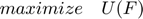


Where  is the total utility, over all possible flows and time. The optimization variable in this problem is the rate matrix
  . The problem data are the rate constraint matrix
  , the utility functions
  , the route matrices
  , the link capacities
  , the delivery contract matrices
  , and the delivery contract quantities
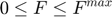
  . The NUMDC problem is a convex optimization problem, and has at most one solution, since the objective is strictly concave. It can however, be infeasible. The above problem can be further formulated using Dual Decomposition, for which the langrangian and the dual function can be defined as:
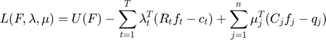
We can solve this dual of the original problem as shown below:

Hence, from the above description, we can clearly say that this dual problem is a convex optimization problem with variables  and
and  . Any feasible point for this dual gives an upper bound on the optimal value of the (primal) NUMDC problem.
3. Data Sources & Assumptions
The data is generated according to the same numerical example in the paper, with the following assumptions:
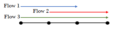
- The network consists of 3 links and 3 flows (i.e. m=n=3), with time horizon T = 10.
- Three delivery contracts are used for this problem, they are:
- Flow 1 must deliver an average rate of at least 4 (per time step) in the period [1,3] and an average rate of at least 10/3 in the period [6,8].
- Flow 2 must deliver an average rate of at least 3 over the period [3,6].
- Flow 3 must deliver an average rate of 1.5 over the period [2,10].
The routes do not vary with time and are shown in the figure below.
4.Solution & Stopping Criteria
Since the problem is formulated as a convex optimization problem, also the Utility functions are logarithmic:  , (for all j and t). This makes possible for us to use the cvx package, which can help us to deal with such sensitive functions.
Proposed Solution
Based on the paper, we described a simple distributed algorithm for solving the langrange dual  of the primal problem. We start with any nonnegative
  …….,
…….,  , and any nonnegative
  ……,
……,  , and repeatedly carry out the update.


where,  and
and 
Also,  is the step size, an algorithm parameter, and
  denotes the positive part of
  , i.e.
![$[0,z]$](ECE602_Mansukh_Muhammad_eq16870080746891744292.png) . The terms
. The terms  ,
,  appearing in the updates are the slacks in the link capacity and contract constraints respectively (and can have negative terms during the algorithm execution). If we stack up these terms, we form exactly the gradient of the dual objective function.
Stopping Criteria
For small enough value of  , this algorithm will converge to a solution of the NUMDC problem, as long as the problem is feasible. This means:


where, , and  is the solution of the primal NUMDC problem and
  is a solution to the dual NUMDC problem.
The stopping criteria is related to the value of , for which the algorithm converges for values of lying between (0, 2 / K), where K is a Lipschitz constant for the dual objective function and is given below:

Where,  ,
,  ,
,  and
and  .
.
- For this example, the Lipshitz constant is calculated and has the value , K=600 for
 , which implies that the proposed algorithm will converge as long as
  .
.
5. Visualization of Results
Using the above mentioned algorithm, we have written the MATLAB code along with their output, in the section below:
cvx_quiet(true);
rand('state', 4);
5.1 Problem Data
% timesteps, links, flows
T = 10;
m = 3;
n = 3;

% routing matrix (is not time varying)
R = [1 0 1;
     1 1 1;
     0 1 1];

% capacity matrix
c_bar = [5;7;5]*ones(1, T); % mean capacities
delc= [1;3;1]*ones(1,T); % deviation +/- around mean
c = c_bar + delc.*(2*rand(m,T)-1);

% flow upper bounds
F_max = 4.5*ones(n,T);

% contracts
C1 = [ones(1,3) zeros(1,7);
      zeros(1,5) ones(1,3) zeros(1,2)];
q1 = [12; 10];

C2 = [zeros(1,2) ones(1,4) zeros(1,4)];
q2 = 12;

C3 = [zeros(1,2) ones(1,8)];
q3 = 12;
5.2 The CVX Solver
fprintf(1,'Solving with CVX...\n')
cvx_begin

    % the rate matrix F
    variable F(n, T)

    %the dual variables
    dual variable lambda
    dual variables mu1 mu2 mu3

    % the DNUM
    maximize    geo_mean(F(:))
    subject to
                % link capacity constraints
                lambda: R*F <= c

                % contract constraints
                mu1: C1*F(1,:)' >= q1
                mu2: C2*F(2,:)' >= q2
                mu3: C3*F(3,:)' >= q3

                % positivity constraints
                F >= 0
                F <= F_max
cvx_end
fprintf(1,'Done!\n\n')
Uopt = sum(log(F(:)));

% convert dual variables for sum(log(F))
lambda = lambda*(n*T)/cvx_optval;
mu1 = mu1*(n*T)/cvx_optval;
mu2 = mu2*(n*T)/cvx_optval;
mu3 = mu3*(n*T)/cvx_optval;

% create P = link_prices - subsidies
link_prices = R'*lambda;
subsidies = [C1'*mu1 C2'*mu2 C3'*mu3];
P = link_prices - subsidies';
Solving with CVX...
Done!
5.3 Dual Decomposition Solution
alpha = 0.01; %step size
Fdd = zeros(n,T);
lambda_dd = zeros(m,T);
mu1_dd = zeros(2,1); mu2_dd = 0; mu3_dd = 0;

fprintf(1,'Solving via Dual Decomposition...\n')
DDiters = 500;
for iter = 1:DDiters
    % create P = link_prices - subsidies
    link_prices = R'*lambda_dd;
    subsidies = [C1'*mu1_dd C2'*mu2_dd C3'*mu3_dd];
    P_dd = link_prices - subsidies';

    % update flows
    Fdd = min(1./P_dd,F_max);
    Fdd(find(P_dd<=0)) = F_max(find(P_dd<=0));
    L(iter) = sum(log(Fdd(:)));

    % update lambda
    cap_slack = c - R*Fdd;
    cap_viols(iter) = max(max(0,-cap_slack(:)));
    L(iter) = L(iter) + sum(sum(lambda_dd.*cap_slack));
    lambda_dd = max(lambda_dd-alpha*cap_slack,0);

    % update mu
    contr_slack1 = C1*Fdd(1,:)'-q1;
    contr_slack2 = C2*Fdd(2,:)'-q2;
    contr_slack3 = C3*Fdd(3,:)'-q3;
    contr_slacks = [contr_slack1; contr_slack2; contr_slack3];
    contr_viols(iter) = max(max(0,-contr_slacks));
    L(iter) = L(iter)+[mu1_dd; mu2_dd; mu3_dd]'*contr_slacks;
    mu1_dd = max(0,mu1_dd-alpha*contr_slack1);
    mu2_dd = max(0,mu2_dd-alpha*contr_slack2);
    mu3_dd = max(0,mu3_dd-alpha*contr_slack3);
end
fprintf(1,'Done!\n\n')

% compare the two solutions
diff_F = norm(F-Fdd,'fro');
diff_lambda = norm(lambda-lambda_dd,'fro')
diff_mu = norm([mu1;mu2;mu3]-[mu1_dd;mu2_dd;mu3_dd]);
fprintf(1,'||F - Fdd|| = %3.3f, ||lambda - lambda_dd|| = %3.3f, ||mu-mu_dd|| = %3.3f\n\n',...
    diff_F,diff_lambda,diff_mu);
Solving via Dual Decomposition...
Done!


diff_lambda =

    0.1349

||F - Fdd|| = 0.103, ||lambda - lambda_dd|| = 0.135, ||mu-mu_dd|| = 0.029
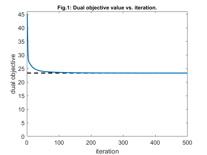
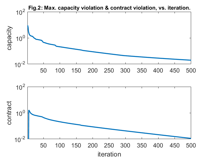
5.4.1 Code for Graphs 2 & 3 of the Paper
% convergence plot
figure
plot(1:DDiters, Uopt*ones(1,DDiters),'k--','linewidth',2); hold on;
set(gca,'FontSize',12);
plot(L,'linewidth',2);
xlabel('iteration');
ylabel('dual objective');
title ('Fig.1: Dual objective value vs. iteration.','FontSize',11)
axis([0 DDiters 0 ceil(max(L))])
box on;
print -depsc ubound.eps

% violation plots
figure
cap_viols(find(cap_viols==0))=1e-4;
subplot(2,1,1);
semilogy(1:DDiters, cap_viols, 'linewidth',2);
set(gca,'FontSize',12);
ylabel('capacity');
title ('Fig.2: Max. capacity violation & contract violation, vs. iteration.','FontSize',11)
axis([1 DDiters 1e-2 1e2]);
box on;

contr_viols(find(contr_viols==0))=1e-4;
subplot(2,1,2);
semilogy(1:DDiters, contr_viols, 'linewidth',2);
set(gca,'FontSize',12);
xlabel('iteration');
ylabel('contract');
axis([1 DDiters 1e-2 1e2]);
box on;
print -depsc violations.eps
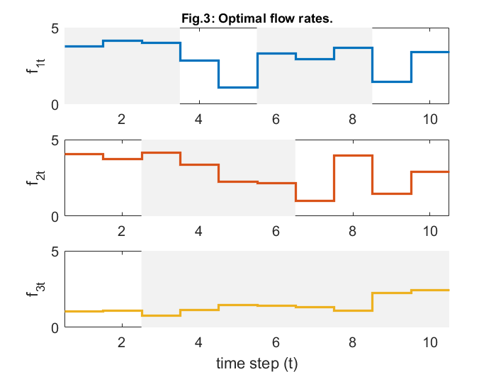
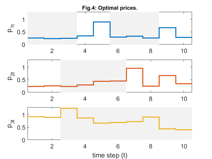
5.4.2 Code for Graphs 4 & 5 of the Paper
In both the figures, the delivery contract periods are shown as shaded regions in the graph.
% plot optimal rates
figure; colors = get(gca,'ColorOrder');
v_max = ceil(max(F(:)));
subplot(3,1,1); hold on
fill([0 3.5 3.5 0],[0 0 v_max v_max],0.95*[1 1 1],'EdgeColor','none');
fill([5.5 8.5 8.5 5.5],[0 0 v_max v_max],0.95*[1 1 1],'EdgeColor','none');
stairs(0.5:1:T+.5, [F(1,:) F(1,end)],'-','Color',colors(1,:),'LineWidth',2);
set(gca,'FontSize',12);
ylabel('f_{1t}');
title ('Fig.3: Optimal flow rates.','FontSize',11)
axis([.5 T+.5 0 v_max]);
box on;

subplot(3,1,2); hold on
fill([2.5 6.5 6.5 2.5],[0 0 v_max v_max],0.95*[1 1 1],'EdgeColor','none');
stairs(0.5:1:T+.5, [F(2,:) F(2,end)],'-','Color',colors(2,:),'LineWidth',2);
set(gca,'FontSize',12);
ylabel('f_{2t}');
axis([.5 T+.5 0 v_max]);
box on;

subplot(3,1,3); hold on
fill([2.5 10.5 10.5 2.5],[0 0 v_max v_max],0.95*[1 1 1],'EdgeColor','none');
stairs(0.5:1:T+.5, [F(3,:) F(3,end)],'-','Color',colors(3,:),'LineWidth',2);
set(gca,'FontSize',12);
ylabel('f_{3t}');
axis([.5 T+.5 0 v_max]);
xlabel('time step (t)');
box on;
print -depsc rate.eps

% plot flow prices
figure; colors = get(gca,'ColorOrder');
v_max = ceil(max(10*P(:)))/10;
v_min = min(0,floor(min(10*P(:)))/10);
subplot(3,1,1); hold on
fill([0 3.5 3.5 0],[v_min v_min v_max v_max],0.95*[1 1 1],'EdgeColor','none');
fill([5.5 8.5 8.5 5.5],[v_min v_min v_max v_max],0.95*[1 1 1],'EdgeColor','none');
stairs(0.5:1:T+.5, [P(1,:) P(1,end)],'-','Color',colors(1,:),'LineWidth',2);
set(gca,'FontSize',12);
ylabel('p_{1t}');
title('Fig.4: Optimal prices.','FontSize',11)
axis([.5 T+.5 v_min v_max]);
box on;

subplot(3,1,2); hold on
fill([2.5 6.5 6.5 2.5],[v_min v_min v_max v_max],0.95*[1 1 1],'EdgeColor','none');
stairs(0.5:1:T+.5, [P(2,:) P(2,end)],'-','Color',colors(2,:),'LineWidth',2);
set(gca,'FontSize',12);
ylabel('p_{2t}');
axis([.5 T+.5 v_min v_max]);
box on;

subplot(3,1,3); hold on
fill([2.5 10.5 10.5 2.5],[v_min v_min v_max v_max],0.95*[1 1 1],'EdgeColor','none');
stairs(0.5:1:T+.5, [P(3,:) P(3,end)],'-','Color',colors(3,:),'LineWidth',2);
set(gca,'FontSize',12);
ylabel('p_{3t}');
axis([.5 T+.5 v_min v_max]);
xlabel('time step (t)');
box on;
print -depsc prices.eps
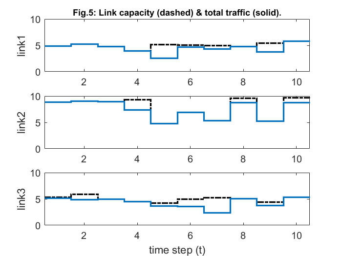
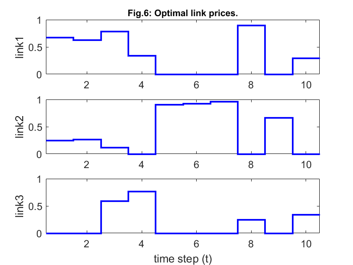
5.4.3 Code for Graphs 6 & 7 of the Paper
% plot link traffic
traffic = R*F; v_max = ceil(max(c(:)));
figure; subplot(3,1,1); hold on;
stairs([0.5:1:T+.5],[c(1,:) c(1,end)],'k-.','LineWidth',2);
stairs([0.5:1:T+.5],[traffic(1,:) traffic(1,end)],'LineWidth',2);
ylabel('link1');
axis([0.5 T+0.5 0 v_max]);
set(gca,'FontSize',12);
title('Fig.5: Link capacity (dashed) & total traffic (solid).','FontSize',11)
box on;

subplot(3,1,2); hold on;
stairs([0.5:1:T+.5],[c(2,:) c(2,end)],'k-.','LineWidth',2);
stairs([0.5:1:T+.5],[traffic(2,:) traffic(2,end)],'LineWidth',2);
ylabel('link2');
axis([0.5 T+0.5 0 v_max]);
set(gca,'FontSize',12);
box on;

subplot(3,1,3); hold on;
stairs([0.5:1:T+.5],[c(3,:) c(3,end)],'k-.','LineWidth',2);
stairs([0.5:1:T+.5],[traffic(3,:) traffic(3,end)],'LineWidth',2);
ylabel('link3');
axis([0.5 T+0.5 0 v_max]);
set(gca,'FontSize',12);
box on;
xlabel('time step (t)');
print -depsc linktraffic.eps

% plot link prices
v_max = ceil(10*max(lambda(:)))/10;
figure; subplot(3,1,1); hold on;
stairs([0.5:1:T+.5],[lambda(1,:) lambda(1,end)],'b-','LineWidth',2);
ylabel('link1');
axis([0.5 T+0.5 0 v_max]);
set(gca,'FontSize',12);
title('Fig.6: Optimal link prices.','FontSize',11)
box on;

subplot(3,1,2); hold on;
stairs([0.5:1:T+.5],[lambda(2,:) lambda(2,end)],'b-','LineWidth',2);
ylabel('link2');
axis([0.5 T+0.5 0 v_max]);
set(gca,'FontSize',12);
box on;

subplot(3,1,3); hold on;
stairs([0.5:1:T+.5],[lambda(3,:) lambda(3,end)],'b-','LineWidth',2);
ylabel('link3');
axis([0.5 T+0.5 0 v_max]);
set(gca,'FontSize',12);
xlabel('time step (t)');
box on;
print -depsc lambda.eps
6. Result Analysis & Conclusion
This report deals with solving of a network utility maximization problem with delivery contract constraints (NUMDC). This is accomplished with the help of a distributed algorithm, which is based on dual decomposition which also established its convergence. The convergence can be confirmed from figures 1 and 2. Figure 3 and 4, on the other hand, tell us that the flow rates generally increase during their contract periods (shaded region) and are generally lower outside contract periods. While, the optimal prices get reduced in this shaded region (in order to encourage increased flow), and are higher elsewhere. Also, these optimal link prices will drop to zero, whenever the link is operating under full capacity as observed from figure 6.
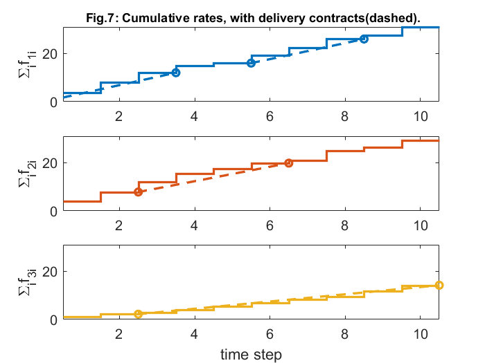
The following figure illustrates the cumulative for each flow with respect to time. The delivey contracts are shown as titlted line segments (dashed), with horizontal span showing the delivery period, and height showing required delivery quantity. For successful delivery of information across the network, this cumulative rate should lie above the righthand endpoint of the line segment.
In a nutshell, from the above analysis of the paper, it can be rightfully said that our results are in full agreement with the ones published by the authors. This was made successful with the help of CVX toolbox which allowed us to solve the problem and reproduce the results. Although, the distributed algorithm requires all rates, prices and updates to occur synchronously. We could also use an incremental subgradient method to solve the NUMDC problem, then we would obtain an algorithm in which updates can occur asynchronously, still with guaranteed convergence.
7. Links & References
- Trichakis N., Zymnis A. & Boyd S. (2008), "Dynamix Network Utility Maximization with Delivery Contracts". IFAC: 2907-12.
- Wei E., Ozdaglar A., Eryilmaz A. & Jadbabaie A. (2010), "A Distributed Newton for Dynamic Network Utility Maximization with Delivery Contracts". Cornell University Press.
- Grant M. & Boyd S. CVX: Matlab software for disciplined convex programming, version 2.0 beta. http://cvxr.com/cvx, September 2013.