ECE602 project: Robust Adaptive Beamforming Using Worst-Case Performance Optimization: A Solution to the Signal Mismatch Problem
Finished by Kaige Qu (20661156)
Contents
- I. Background of beamforming and the optimal solution
- II. Three existing beamforming approaches
- III. Proposed robust beamforming solution
- IV. Simulation results of the optimal, SMI, LSMI, eigenspace-based and the proposed beamformers for three example senarios
- IV-A. Output SINR versus training sample size N, with constant SNR=-10dB
- IV-B. Output SINR versus SNR, with constant sample size N = 30
- IV-C. Output SINR versus
 in the proposed solution for the first example
I. Background of beamforming and the optimal solution

- Background of beamforming
The output of a narrowband beamformer is given by  , in which
 ![$\textbf{x}(k)=[x_1(k),...,x_M(k)]^T$](project_publish_eq00236863400328806847.png) is the complex vector of array observations,
is the complex vector of array observations, ![$\textbf{w}=[w_1,...,w_M]^T$](project_publish_eq08157895808925301105.png) is the complex vector of beamformer weights, and
is the complex vector of beamformer weights, and  is the number of array sensors.
The observation (training snapshot) vector is given by

where  ,
,  , and
, and  are the desired signal, interference, and noise components, respectively. Here,
  is the signal waveform, and
  is the signal steering vector.
The weight vector can be found from the maximum of the signal-to-interference-plus-noise ratio
where ![$\textbf{R}_{i+n}=E[(\textbf{i}(k)+\textbf{n}(k))(\textbf{i}(k)+\textbf{n}(k))^H]$](project_publish_eq16577883944719253037.png) is the exact interference-plus-noise covariance matrix, and
is the exact interference-plus-noise covariance matrix, and  is the signal power.
However, in the mismatched case, the presumed and actual signal steering vectors and  are different. Then the evaluation of SINR after solving the beamforming algorithm based on maximizing (2) should then conform to (3) rather than (2).

- The optimal solution (Minimum Variance Distortionless Response(MVDR) Beamformer)
The maximization of (2) is equivalent to solve the following optimization problem

The solution of (4) is  , where
  is the normalization constant that does not affect the output SINR (2) and, therefore, will be omitted in the following text.
So the solution of optimal beamformer is
And the signal-to-interference-plus-noise ratio is

in the case of exactly known signal steering vector , and

in the case of mismatch.
II. Three existing beamforming approaches
In practical applications, the exact interference-plus-noise covariance matrix  is unavailable (although in simulation we can calculate it). Therefore, the sample covariance matrix
  (8) is used instead for the beamforming algorithm. The three exsting beamforming algorithms listed below are all based on . Here, please note that is still used for evaluating the SINR according to (2) or (3).
In (8),  is the number of training snapshots.
- The Sample Matrix Inversion (SMI) Beamformer
The solution of SMI beamformer is given by
- The Loaded SMI (LSMI) Beamformer
LSMI beamformer is one robust modification of the SMI algorithm. In LSMI, the conventional sample covariance matrix is replaced by the diagonally loaded covariance matrix  . The solution of LSMI beamformer is given by

- The Eigenspace-based Beamformer
The eigenspace-based beamformer is also a robust adaptive beamforming approach. The key idea is to use the projection of the presumed steering vector onto the sample signal-plus-interference subspace, instead of itself for beamforming. The eigen-decomposition of yields
where  contains
  signal-plus-interference subspace eigenvectors of , and the diagonal matrix
  contains the corresponding eigenvalues. Similarly, the matrix
  contains the
  noise-subspace eigenvectors of , whereas the diagonal matrix
  is built from the corresponding eigenvalues.
The solution of eigenspace-based beamformer is given by
III. Proposed robust beamforming solution
First, the actual signal steering vector is assumed to belong to the set  . We impose a constraint for all vectors that belong to
  . That is,
Then, the robust formulation is

Going through several steps, (12) can be rewritten as

where
![$$\breve{\textbf{w}}=[Re\{\textbf{w}\}^T, Im\{\textbf{w}\}^T]^T$$](project_publish_eq04541717451595793121.png)
![$$\breve{\textbf{a}}=[Re\{\textbf{a}\}^T, Im\{\textbf{a}\}^T]^T$$](project_publish_eq02437129809125367405.png)
![$$\bar{\textbf{a}}=[Im\{\textbf{a}\}^T, -Re\{\textbf{a}\}^T]^T$$](project_publish_eq13145647043022416471.png)
![$\breve{\textbf{U}}=[Re\{\textbf{U}\},-Im\{\textbf{U}\};Im\{\textbf{U}\},Re\{\textbf{U}\}]$](project_publish_eq01050206938390299131.png)
This problem is an SOC problem, and can be solved by CVX.
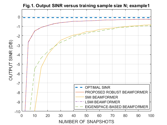
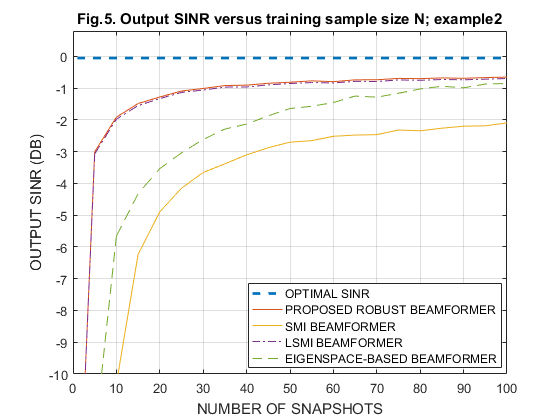
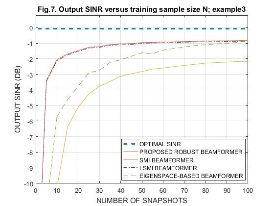
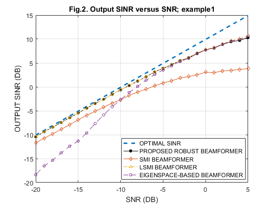
IV. Simulation results of the optimal, SMI, LSMI, eigenspace-based and the proposed beamformers for three example senarios
I have done the simulation for the first three examples in the paper. And the output SINR of the optimal, SMI, LSMI, eigenspace-based and the proposed beamformers are comprared. Three comparisons are done. The first is "Output SINR versus training sample size N, with constant SNR=-10dB". Then comes "Output SINR versus SNR, with constant sample size N = 30". The last is "Output SINR versus in the proposed solution for the first example". The main body of the code is similar, only changing the data inputs. The simulation results are averaged over 200 simulations. As the execution time is too long, I have saved the results and loaded them to plot the figures in this project_publish.m.
The three examples are
- Example 1: Exactly Known Signal Steering Vector
- Example 2: Signal Look Direction Mismatch
- Example 3: Signal Spatial Signature Mismatch Due to Coherent Local Scattering
Different examples provide different . In the code, I comment on the code of the other two examples when doing one of them.
IV-A. Output SINR versus training sample size N, with constant SNR=-10dB
clear all;
%
% parameters
M=10;  % No. of sensors
SNR_dB = -10;
ps = 10^(SNR_dB/10);
tet_no=3; % nominal impinging angle
tet_ac=5; % actual impinging angle(In Example 2)
tet_mean = 3; % mean impinging angle for b1~b4 (in Example 3)
%
% interference generation
tet_I= [30, 50]; % impinging angles of interfering sources
J  = length(tet_I); % No. of interfering sources
a_I = exp(1i*2.0*[0:M-1]'*pi*0.5*sin(tet_I*pi/180.0)); % interfering steering matrix
INR  = 1000; % interference noise ratio
R_I_n=INR*a_I*a_I'+eye(M,M); % ideal interference-plus-noise covariance matrix % used to calculate SINR
%
SINR_SMI=zeros(1,100);% 100 different N (snapshots)
SINR_eig=zeros(1,100);
SINR_PRO=zeros(1,100);
SINR_LSMI=zeros(1,100);
%
% No. of simulations=200
for loop=1:200;
  a = exp(1i*2.0*[0:M-1]'*pi*0.5*sin(tet_no*pi/180.0));% nominal a
%   generation of actual signal steering vector a_tilde
%   Example 1: Exactly Known Signal Steering Vector
  a_tilde = a;
%   Example 2: Signal Look Direction Mismatch
%     a_tilde = exp(1i*2.0*[0:M-1]'*pi*0.5*sin(tet_ac*pi/180.0));
%   Example 3: Signal Signature Mismatch Due to Coherent Local Scattering
%     var=4;
%     b1 = exp(1i*2.0*[0:M-1]'*pi*0.5*sin((tet_mean+rand*sqrt(3*var))*pi/180.0)); % better to use randn for Gaussian noise
%     b2 = exp(1i*2.0*[0:M-1]'*pi*0.5*sin((tet_mean+rand*sqrt(3*var))*pi/180.0));
%     b3 = exp(1i*2.0*[0:M-1]'*pi*0.5*sin((tet_mean+rand*sqrt(3*var))*pi/180.0));
%     b4 = exp(1i*2.0*[0:M-1]'*pi*0.5*sin((tet_mean+rand*sqrt(3*var))*pi/180.0));
%     psi1 = 2*rand*pi; psi2 = 2*rand*pi; psi3 = 2*rand*pi; psi4 = 2*rand*pi;
%     a_tilde = a + exp(1i*psi1)*b1 + exp(1i*psi2)*b2 + exp(1i*psi3)*b3 + exp(1i*psi4)*b4; % actual a (tilde)
  a_tilde = sqrt(10)*a_tilde/norm(a_tilde)';
  %
  Ncount=0;
  for N=[1 5 10 15 20 25 30 35 40 45 50 55 60 65 70 75 80 85 90 95 100] % No. of snapshots
      Ncount=Ncount+1;
      R_hat = zeros(M);
      for l=1:N
          s=(randn(1,1) + 1i*randn(1,1))*sqrt(ps)*sqrt(0.5);  % signal waveform
          Is = (randn(J,1) + 1i*randn(J,1)).*sqrt(INR)'*sqrt(0.5); % interference waveform
          n = (randn(M,1) + 1i*randn(M,1))*sqrt(0.5); % noise
          x = a_I*Is + s*a_tilde + n; % snapshot with signal
          R_hat = R_hat + x*x';
      end
      R_hat=R_hat/N;  % sample covariance matrix
      %
      % sample matrix inversion (SMI) algorithm
      w_SMI=inv(R_hat)*a;
      %
      % LSMI algorithm
      R_dl_hat = R_hat + eye(M,M)*10;
      w_LSMI=inv(R_dl_hat)*a;
      %
      % eigenspace-based robust beamformer
      [RR,D]=eig(R_hat);   % eigenvalue decomposition of covariance matrix
      RR_subs=RR(:,M-2:M);
      as_new=[RR_subs,zeros(M,M-3)]*a;  % projection of waveform to SIGNAL and INTERFERENCE space
      ws_EIG=inv(R_hat)*as_new;
      %
      % proposed robust beamformer using worst-case performance optimization
      R_hat = R_hat + eye(M,M)*0.01; % diagonal loading
      U=chol(R_hat);  % Cholesky factorization
      U_bowl=[real(U),-imag(U);imag(U),real(U)];  % 'U_bowl' defined based on 'U'
      M2 = 2*M;
      a_bowl=[real(a);imag(a)];  % 'a_bowl' difined based on 'a'
      a_bar = [imag(a);-real(a)];
      FT = [1,zeros(1,M2);zeros(M2,1),U_bowl;0,a_bowl';zeros(M2,1),3*eye(M2,M2);0,a_bar'];
      cvx_begin
          variable y(M2+1,1)
          minimize (y(1))
          c = FT*y;
          subject to
              c(1) >= norm(c(2:M2+1));
              c(M2+2)-1 >= norm(c(M2+3:2*M2+2));
              c(2*M2+3) == 0;
      cvx_end
      w_PRO_bowl = y(2:21);
      w_PRO = w_PRO_bowl(1:10) + 1i * w_PRO_bowl(11:20);
      %
      SINR_SMI_v(Ncount) = ps * (abs(w_SMI'*a_tilde) * abs(w_SMI'*a_tilde)) / abs(w_SMI'*R_I_n*w_SMI);  % SINR
      SINR_LSMI_v(Ncount) = ps * (abs(w_LSMI'*a_tilde) * abs(w_LSMI'*a_tilde)) / abs(w_LSMI'*R_I_n*w_LSMI);
      SINR_EIG_v(Ncount) = ps * (abs(ws_EIG'*a_tilde) * abs(ws_EIG'*a_tilde)) / abs(ws_EIG'*R_I_n*ws_EIG);
      SINR_PRO_v(Ncount) = ps * (abs(w_PRO'*a_tilde) * abs(w_PRO'*a_tilde)) / abs(w_PRO'*R_I_n*w_PRO); % SINR for robust beamformer
      SINR_opt(Ncount) = ps * a_tilde' * inv(R_I_n) * a_tilde;
  end
  SINR_SMI     = ((loop-1)/loop)*SINR_SMI + (1/loop)*SINR_SMI_v; % just average
  SINR_LSMI    = ((loop-1)/loop)*SINR_LSMI + (1/loop)*SINR_LSMI_v;
  SINR_eig     = ((loop-1)/loop)*SINR_eig + (1/loop)*SINR_EIG_v;
  SINR_PRO   = ((loop-1)/loop)*SINR_PRO + (1/loop)*SINR_PRO_v;
end;
save('Fig1_for_EX1','SINR_opt','SINR_SMI', 'SINR_LSMI','SINR_eig','SINR_PRO')
% save('Fig5_for_EX2','SINR_opt','SINR_SMI', 'SINR_LSMI','SINR_eig','SINR_PRO')
% save('Fig7_for_EX3','SINR_opt','SINR_SMI', 'SINR_LSMI','SINR_eig','SINR_PRO')
N_sa=[1 5 10 15 20 25 30 35 40 45 50 55 60 65 70 75 80 85 90 95 100];
Fig_No = [1 5 7];
load('Fig1_for_EX1'); % Ex1
SINR_SMI_m(1,:) = SINR_SMI;
SINR_eig_m(1,:) = SINR_eig;
SINR_PRO_m(1,:) = SINR_PRO;
SINR_LSMI_m(1,:) = SINR_LSMI;
SINR_opt_m(1,:) = SINR_opt;
load('Fig5_for_EX2'); % Ex2
SINR_SMI_m(2,:) = SINR_SMI;
SINR_eig_m(2,:) = SINR_eig;
SINR_PRO_m(2,:) = SINR_PRO;
SINR_LSMI_m(2,:) = SINR_LSMI;
SINR_opt_m(2,:) = SINR_opt;
load('Fig7_for_EX3'); % Ex3
SINR_SMI_m(3,:) = SINR_SMI;
SINR_eig_m(3,:) = SINR_eig;
SINR_PRO_m(3,:) = SINR_PRO;
SINR_LSMI_m(3,:) = SINR_LSMI;
SINR_opt_m(3,:) = SINR_opt;
for i = 1:3
    figure
    plot(N_sa,10*log10(abs(SINR_opt_m(i,:))),'--','LineWidth',2);
    hold on;
    plot(N_sa,10*log10(abs(SINR_PRO_m(i,:))),'-');
    hold on;
    plot(N_sa,10*log10(abs(SINR_SMI_m(i,:))),'-');
    hold on;
    plot(N_sa,10*log10(abs(SINR_LSMI_m(i,:))),'-.');
    hold on;
    plot(N_sa,10*log10(abs(SINR_eig_m(i,:))),'--');
    hold off;
    grid on;
    gca=legend('OPTIMAL SINR','PROPOSED ROBUST BEAMFORMER','SMI BEAMFORMER',...
            'LSMI BEAMFORMER','EIGENSPACE-BASED BEAMFORMER');
    set( gca, 'Position', [0.495 0.14 0.35 0.17]);
    axis([0,100,-10,0.8]);
    xlabel('NUMBER OF SNAPSHOTS');
    ylabel('OUTPUT SINR (DB)');
    title(['Fig.',num2str(Fig_No(i)),'. Output SINR versus training sample size N; example',num2str(i)]);
end
clear all;
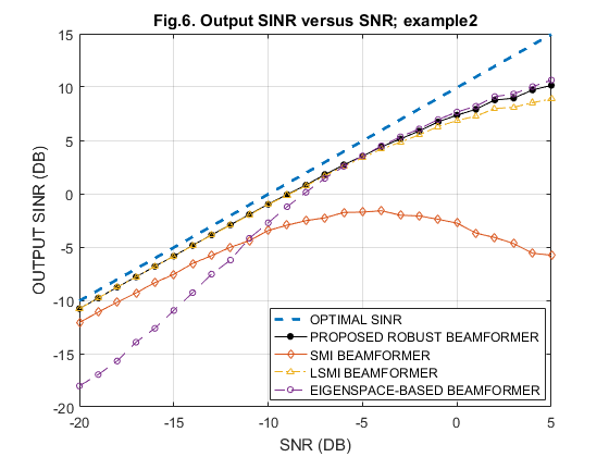
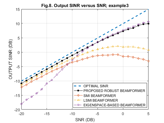
IV-B. Output SINR versus SNR, with constant sample size N = 30
clear all;
%
% parameters
N=30; % No. of snapshots
M=10;  % No. of sensors
tet_no=3; % nominal impinging angle
tet_ac=5; % actual impinging angle(In Example 2)
tet_mean = 3; % mean impinging angle for b1~b4 (in Example 3)
%
% interference generation
tet_I= [30, 50]; % impinging angles of interfering sources
J  = length(tet_I); % No. of interfering sources
a_I = exp(1i*2.0*[0:M-1]'*pi*0.5*sin(tet_I*pi/180.0)); % interfering steering matrix
INR  = 1000; % interference noise ratio
R_I_n=INR*a_I*a_I'+eye(M,M); % ideal interference-plus-noise covariance matrix % used to calculate SINR
%
SNR_dB = [-20 -19 -18 -17 -16 -15 -14 -13 -12 -11 -10 -9 -8 -7 ...
      -6 -5 -4 -3 -2 -1 0 1 2 3 4 5];
for i=1:length(SNR_dB)
  SNR(i) = 10^(SNR_dB(i)/10);
end
%
SINR_SMI=zeros(1,length(SNR));
SINR_eig=zeros(1,length(SNR));
SINR_PRO=zeros(1,length(SNR));
SINR_LSMI=zeros(1,length(SNR));
%
% No. of simulations=200
for loop=1:200;
  a = exp(1i*2.0*[0:M-1]'*pi*0.5*sin(tet_no*pi/180.0));% nominal a
% % generation of actual signal steering vector a_tilde
% % Example 1: Exactly Known Signal Steering Vector
  a_tilde = a;
%  % Example 2: Signal Look Direction Mismatch
%     a_tilde = exp(1i*2.0*[0:M-1]'*pi*0.5*sin(tet_ac*pi/180.0));
%  % Example 3: Signal Signature Mismatch Due to Coherent Local Scattering
%     var=4;
%     b1 = exp(1i*2.0*[0:M-1]'*pi*0.5*sin((tet_mean+rand*sqrt(3*var))*pi/180.0)); % better to use randn for Gaussian noise
%     b2 = exp(1i*2.0*[0:M-1]'*pi*0.5*sin((tet_mean+rand*sqrt(3*var))*pi/180.0));
%     b3 = exp(1i*2.0*[0:M-1]'*pi*0.5*sin((tet_mean+rand*sqrt(3*var))*pi/180.0));
%     b4 = exp(1i*2.0*[0:M-1]'*pi*0.5*sin((tet_mean+rand*sqrt(3*var))*pi/180.0));
%     psi1 = 2*rand*pi; psi2 = 2*rand*pi; psi3 = 2*rand*pi; psi4 = 2*rand*pi;
%     a_tilde = a + exp(1i*psi1)*b1 + exp(1i*psi2)*b2 + exp(1i*psi3)*b3 + exp(1i*psi4)*b4; % actual a (tilde)
  a_tilde = sqrt(10)*a_tilde/norm(a_tilde)';
  %
  Ncount=0;
  %
  for ps=SNR;
      Ncount=Ncount+1;
      R_hat = zeros(M);
      for l=1:N
          s=(randn(1,1) + 1i*randn(1,1))*sqrt(ps)*sqrt(0.5);  % signal waveform
          Is = (randn(J,1) + 1i*randn(J,1)).*sqrt(INR)'*sqrt(0.5); % interference waveform
          n = (randn(M,1) + 1i*randn(M,1))*sqrt(0.5); % noise
          x = a_I*Is + s*a_tilde + n; % snapshot with signal
          R_hat = R_hat + x*x';
      end
      R_hat=R_hat/N;  % sample covariance matrix
      %
      % sample matrix inversion (SMI) algorithm
      w_SMI=inv(R_hat)*a;
      %
      % LSMI algorithm
      R_dl_hat = R_hat + eye(M,M)*10;
      w_LSMI=inv(R_dl_hat)*a;
      %
      % eigenspace-based robust beamformer
      [RR,D]=eig(R_hat);   % eigenvalue decomposition of covariance matrix
      RR_subs=RR(:,M-2:M);
      as_new=[RR_subs,zeros(M,M-3)]*a;  % projection of waveform to SIGNAL and INTERFERENCE space
      ws_EIG=inv(R_hat)*as_new;
      %
      % proposed robust beamformer using worst-case performance optimization
      R_hat = R_hat + eye(M,M)*0.01; % diagonal loading
      U=chol(R_hat);  % Cholesky factorization
      U_bowl=[real(U),-imag(U);imag(U),real(U)];  % 'U_bowl' defined based on 'U'
      M2 = 2*M;
      a_bowl=[real(a);imag(a)];  % 'a_bowl' difined based on 'a'
      a_bar = [imag(a);-real(a)];
      FT = [1,zeros(1,M2);zeros(M2,1),U_bowl;0,a_bowl';zeros(M2,1),3*eye(M2,M2);0,a_bar'];
      cvx_begin
          variable y(M2+1,1)
          minimize (y(1))
          c = FT*y;
          subject to
              c(1) >= norm(c(2:M2+1));
              c(M2+2)-1 >= norm(c(M2+3:2*M2+2));
              c(2*M2+3) == 0;
      cvx_end
      w_PRO_bowl = y(2:21);
      w_PRO = w_PRO_bowl(1:10) + 1i * w_PRO_bowl(11:20);
      %
      SINR_SMI_v(Ncount) = ps * (abs(w_SMI'*a_tilde) * abs(w_SMI'*a_tilde)) / abs(w_SMI'*R_I_n*w_SMI);  % SINR
      SINR_LSMI_v(Ncount) = ps * (abs(w_LSMI'*a_tilde) * abs(w_LSMI'*a_tilde)) / abs(w_LSMI'*R_I_n*w_LSMI);
      SINR_EIG_v(Ncount) = ps * (abs(ws_EIG'*a_tilde) * abs(ws_EIG'*a_tilde)) / abs(ws_EIG'*R_I_n*ws_EIG);
      SINR_PRO_v(Ncount) = ps * (abs(w_PRO'*a_tilde) * abs(w_PRO'*a_tilde)) / abs(w_PRO'*R_I_n*w_PRO); % SINR for robust beamformer
      SINR_opt(Ncount) = ps * a_tilde' * inv(R_I_n) * a_tilde;
  end
  SINR_SMI     = ((loop-1)/loop)*SINR_SMI + (1/loop)*SINR_SMI_v; % just average
  SINR_LSMI    = ((loop-1)/loop)*SINR_LSMI + (1/loop)*SINR_LSMI_v;
  SINR_eig     = ((loop-1)/loop)*SINR_eig + (1/loop)*SINR_EIG_v;
  SINR_PRO   = ((loop-1)/loop)*SINR_PRO + (1/loop)*SINR_PRO_v;
end;
save('Fig2_for_EX1','SINR_opt','SINR_SMI', 'SINR_LSMI','SINR_eig','SINR_PRO') % Ex1
% save('Fig6_for_EX2','SINR_opt','SINR_SMI', 'SINR_LSMI','SINR_eig','SINR_PRO') % Ex2
% save('Fig8_for_EX3','SINR_opt','SINR_SMI', 'SINR_LSMI','SINR_eig','SINR_PRO') % Ex3
SNR_dB = [-20 -19 -18 -17 -16 -15 -14 -13 -12 -11 -10 -9 -8 -7 ...
        -6 -5 -4 -3 -2 -1 0 1 2 3 4 5];
Fig_No = [2 6 8];
load('Fig2_for_EX1'); % Ex1
SINR_SMI_m(1,:) = SINR_SMI;
SINR_eig_m(1,:) = SINR_eig;
SINR_PRO_m(1,:) = SINR_PRO;
SINR_LSMI_m(1,:) = SINR_LSMI;
SINR_opt_m(1,:) = SINR_opt;
load('Fig6_for_EX2'); % Ex2
SINR_SMI_m(2,:) = SINR_SMI;
SINR_eig_m(2,:) = SINR_eig;
SINR_PRO_m(2,:) = SINR_PRO;
SINR_LSMI_m(2,:) = SINR_LSMI;
SINR_opt_m(2,:) = SINR_opt;
load('Fig8_for_EX3'); % Ex3
SINR_SMI_m(3,:) = SINR_SMI;
SINR_eig_m(3,:) = SINR_eig;
SINR_PRO_m(3,:) = SINR_PRO;
SINR_LSMI_m(3,:) = SINR_LSMI;
SINR_opt_m(3,:) = SINR_opt;
for i = 1:3
    figure;
    plot(SNR_dB,10*log10(abs(SINR_opt_m(i,:))),'--','LineWidth',2);
    hold on;
    plot(SNR_dB,10*log10(abs(SINR_PRO_m(i,:))),'k-o','MarkerFaceColor','k', 'MarkerSize',4);
    hold on;
    plot(SNR_dB,10*log10(abs(SINR_SMI_m(i,:))),'-d','MarkerSize',4);
    hold on;
    plot(SNR_dB,10*log10(abs(SINR_LSMI_m(i,:))),'-.^','MarkerSize',4);
    hold on;
    plot(SNR_dB,10*log10(abs(SINR_eig_m(i,:))),'--o','MarkerSize',4);
    hold off;
    grid on;
    gca=legend('OPTIMAL SINR','PROPOSED ROBUST BEAMFORMER','SMI BEAMFORMER',...
            'LSMI BEAMFORMER','EIGENSPACE-BASED BEAMFORMER');
    set( gca, 'Position', [0.495 0.14 0.35 0.17]);
    xlabel('SNR (DB)')
    ylabel('OUTPUT SINR (DB)')
    title(['Fig.',num2str(Fig_No(i)),'. Output SINR versus SNR; example',num2str(i)]);
end
clear all;
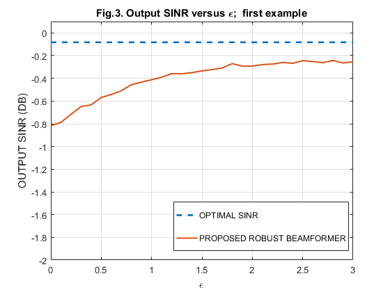
IV-C. Output SINR versus in the proposed solution for the first example
clear all;
M=10;  % No. of sensors
N=100; % No. of snapshots
SNR_dB = -10;
ps = 10^(SNR_dB/10);
tet_no=3; % nominal impinging angle
tet_I= [30, 50]; % impinging angles of interfering sources
J  = length(tet_I); % No. of interfering sources
a_I = exp(1i*2.0*[0:M-1]'*pi*0.5*sin(tet_I*pi/180.0)); % interfering steering matrix
INR  = 1000; % interference noise ratio
R_I_n=INR*a_I*a_I'+eye(M,M); % ideal interference-plus-noise covariance matrix % used to calculate SINR
%
factor = [0:0.1:3];
SINR_PRO=zeros(1,length(factor));
%
% No. of simulations=200
for loop=1:200;
  a = exp(1i*2.0*[0:M-1]'*pi*0.5*sin(tet_no*pi/180.0));% nominal a
  a_tilde = a; % actual a (tilde)
  a_tilde = sqrt(10)*a_tilde/norm(a_tilde)';
  Ncount=0;
  for factor = 0:0.1:3
      Ncount=Ncount+1;
      R_hat = zeros(M);
      for l=1:N
          s=(randn(1,1) + 1i*randn(1,1))*sqrt(ps)*sqrt(0.5);  % signal waveform
          Is = (randn(J,1) + 1i*randn(J,1)).*sqrt(INR)'*sqrt(0.5); % interference waveform
          n = (randn(M,1) + 1i*randn(M,1))*sqrt(0.5); % noise
          x = a_I*Is + s*a_tilde + n; % snapshot with signal
          R_hat = R_hat + x*x';
      end
      R_hat=R_hat/N;  % sample covariance matrix
      %
      % proposed robust beamformer using worst-case performance optimization
      R_hat = R_hat + eye(M,M)*0.01; % diagonal loading
      U=chol(R_hat);  % Cholesky factorization
      U_bowl=[real(U),-imag(U);imag(U),real(U)];  % 'U_bowl' defined based on 'U'
      M2 = 2*M;
      a_bowl=[real(a);imag(a)];  % 'a_bowl' difined based on 'a'
      a_bar = [imag(a);-real(a)];
      FT = [1,zeros(1,M2);zeros(M2,1),U_bowl;0,a_bowl';zeros(M2,1),factor*eye(M2,M2);0,a_bar'];
      cvx_begin
          variable y(M2+1,1)
          minimize (y(1))
          c = FT*y;
          subject to
              c(1) >= norm(c(2:M2+1));
              c(M2+2)-1 >= norm(c(M2+3:2*M2+2));
              c(2*M2+3) == 0;
      cvx_end
      w_PRO_bowl = y(2:21);
      w_PRO = w_PRO_bowl(1:10) + 1i * w_PRO_bowl(11:20);
      SINR_PRO_v(Ncount) = ps * (abs(w_PRO'*a_tilde) * abs(w_PRO'*a_tilde)) / abs(w_PRO'*R_I_n*w_PRO); % SINR for robust beamformer
      SINR_opt(Ncount) = ps * a_tilde' * inv(R_I_n) * a_tilde;
  end
  SINR_PRO   = ((loop-1)/loop)*SINR_PRO + (1/loop)*SINR_PRO_v;
end;
save('Fig3_for_EX1','SINR_opt','SINR_PRO')
load('Fig3_for_EX1');
figure
plot(0:0.1:3,10*log10(abs(SINR_opt)),'--','LineWidth',2);
hold on;
plot(0:0.1:3,10*log10(abs(SINR_PRO)),'-','LineWidth',1.5);
hold off;
grid on;
gca=legend('OPTIMAL SINR','PROPOSED ROBUST BEAMFORMER');
set( gca, 'Position', [0.495 0.14 0.35 0.17]);
axis([0,3,-2,0.1]);
xlabel('\epsilon');
ylabel('OUTPUT SINR (DB)');
title('Fig.3. Output SINR versus \epsilon;  first example');