Robust Sampled-Data H-Infinity Control for Vehicle Active Suspension Systems

Nan Wei (20625558)

Kyongjae Woo (20343297)

Yubiao Zhang (20656508)

1. Introduction
2. Problem Formulation
3. Proposed Solution
4. Data Sources
5. Deterministic System Case
6. Nondeterministic System Case
7. Analysis and Conclusions
8. References

1. Introduction

Active suspension systems have been recognized as a demanding approach for its flexibility in its dynamics to provide both ride comfort and performance, which are often conflicting. In the paper, the authors have investigated the feasibility of robust sampled-data $H_{\infty}$ controller [1]. By using an input delay approach, the active suspension system with sampling measurements is transformed into a continuous-time (CT) system with a delay in the state. The transformed CT system has time varying state delay and polytopic parameter uncertainties. The uncertainty problem can be formulated as convex Linear Matrix Inequality(LMI) optimization problem [2].

The purpose of this project is to use cvx convex optimization toolbox [3] to solve the aforementioned LMI optimization problem to construct an optimal sampled-data $H_{\infty}$ controller.

2. Problem Formulation

In the paper [1], the following quater-car model is used to study the performance of the active suspension system.

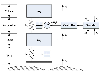
Fig. 1. Schematic of the quarter car model [1].

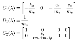
Using input delay approach, this system can be described as

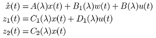
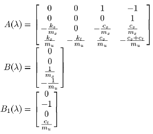
where $x$ is the state variable given in [1], $\omega$ is the disturbance, $z_1$ is the vertical body acceleration which is correlated to the ride comfort, and $z_2$ includes 2 constrained outputs: suspension stroke and relative dynamic tyre load. The matrices are

where $\lambda$ is used to characterize the parameter uncertainty. The parameters in these matrices are explained in Section 4. For such system, it is assumed that the state variables are measuared at discrete time instants, so that the desired state feedback controller can be expressed as the following form,

The objective is to design a gain matrix K such that [1]:

the closed-loop system is asymptotically stable;
given that the initial condition is zero, the closed-loop system guarantees that $\|z_{1}(t)\|_{2}\leq\gamma\|\omega(t)\|_{2}$ for all nonzero $\omega\in L_{2}[0,\infty)$ , where $\gamma>0$ ;
the input and output constraints are guaranteed: $|u(t)|\leq u_{max}$ , and $|\{z_2(t)\}_j|\leq\{z_{2,max}\}_j$ , for any , , and $z_{2,max}=[z_{max}, 1]^T$ .

Note that the norm $\| y(t)\|_2$ for the scalar signal $y(t)$ is defined as $\|y(t)\|_2=\sqrt{\int_{t=0}^{\infty} |y(t|^2 dt}$

3. Proposed Solution

Under the assumption that any two consecutive sampling instants is bounded by some scalar $h(h>0)$ , and with scalars $\gamma>0$ , and $\rho>0$ , the aforementioned problem can be formulated as a convex optimization problem as shown below [1].

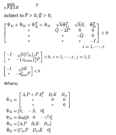
The problem optimizes the scalar $\gamma$ which is an indicator of system performance; a smaller $\gamma$ represents better suspension performance it yields. If a feasible solution to the optimization problem exists, then one can find the optimal gains by $K=\bar{K}P^{-1}$ . A detailed discussion on the proof is out of the scope of this report, and the interested reader is referred to [1] for more information.

4. Data Sources

All of the parameters used in this project are from the paper [1]. The table below summarizes the parameters used and their corresponding values:

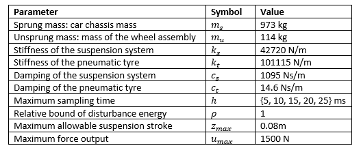
For the nondeterministic case, the suspension system is uncertain in the sprung and usprung masses, while all other parameters are known to be the same as the deterministic case:

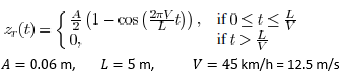
In all simulations, the same disturbance input is used. It is the time derivative of the ground displacement, which is

5. Deterministic System Case

In this case, an example is provided to illustrate the effectiveness of the proposed sampled-data controller design. It considers the nominal system with no parameter uncertainties. The closed-loop response of the sampled-data system with optimal feedback gains is compared with that of a passive system. It is also compared with the simulation result of a system with an optimal controller assuming that measurement and control are performed in continuous-time. The optimal feedback gain for the continuous-time system is obtained from [4].

% Model parameters %%%%%%%%%%%%%%%%%%%%%%%%%%%%%%%%%%%%%%%%%%%%%%%%%%%%%%%%
% Data from Section IV and Table I from the paper
ms=973; % sprung mass: car chassis mass
mu=114; % unsprung mass: mass of wheel assembly
ks=42720;   % stiffness of suspension system
kt=101115;  % stiffness of the pneumatic tyre
cs=1095;    % damping of the suspension system
ct=14.6;    % damping of the pneumatic tyre
% maximum sampling time intervals, from Table II
H=[5e-3,10e-3,15e-3,20e-3,25e-3];
g=9.81; % gravitational constant
rho=1;  % rho is related to the bound of disturbance energy
z_max=0.08; % max allowable suspension stroke
u_max=1500; % max force output
% State Space Matrices %%%%%%%%%%%%%%%%%%%%%%%%%%%%%%%%%%%%%%%%%%%%%%%%%%%%
% These matrices are from Section II of the paper
A=[0,0,1,-1;
   0,0,0,1;
   -ks./ms,0,-cs./ms,cs./ms;
   ks./mu,-kt./mu,cs./mu,-(cs+ct)./mu];
B=[0;0;1./ms;-1./mu];
B1=[0;-1;0;ct./mu];
C1=[-ks./ms,0,-cs./ms,cs./ms];
D1=1./ms;
C2=[1,0,0,0;
    0,kt./(ms+mu)./g,0,0];
gamma_min=[];  % used to record the H-infinity gain for diff sampling times
K=[];   % used to record the optimal gain for diff sampling times
% Optimization %%%%%%%%%%%%%%%%%%%%%%%%%%%%%%%%%%%%%%%%%%%%%%%%%%%%%%%%%%%%
% Run the same optimization for different sampling times
% Formulation given at bottom of Part III
for n=1:length(H)
    h=H(n); % max sampling time for the current optimization
    cvx_begin quiet;
        variable Gamma2;    % Gamma.^2
        variable P_bar(4,4) symmetric;
        variable Q_bar(4,4) symmetric;
        % Note that there is a typo in the paper. S_bar is not a square
        % matrix and cannot be positive definite
        variable S_bar(9,4);
        variable K_bar(1,4);
        % Equation (34)
        Psi_bar1=[A*P_bar+P_bar*A.', B*K_bar, B1;
                  (B*K_bar).', zeros(4,4), zeros(4,1);
                  (B1).', zeros(1,4), zeros(1,1)];
        Psi_bar2=[S_bar, -S_bar, zeros(9,1)];
        Psi_5=-Gamma2.*eye(9);
        Psi_5(1:8,1:8)=zeros(8,8);
        Phi_bar1=[A*P_bar, B*K_bar, B1];
        Phi_bar2=[C1*P_bar, D1*K_bar, 0];
        % Equation (31)
        Mat1=[Psi_bar1+Psi_bar2+Psi_bar2.'+Psi_5, sqrt(h).*Phi_bar1.', ...
                    sqrt(h).*S_bar, Phi_bar2.';
              sqrt(h).*Phi_bar1, Q_bar-2*P_bar, zeros(4,4), zeros(4,1);
              sqrt(h).*S_bar.', zeros(4,4), -Q_bar, zeros(4,1);
              Phi_bar2, zeros(1,4), zeros(1,4), -1];
        % Equation (32) for j=1
        Mat21=[-eye(1), sqrt(rho).*C2(1,:)*P_bar;
              (sqrt(rho).*C2(1,:)*P_bar).', -z_max.^2*P_bar];
        % Equation (32) for j=2
        Mat22=[-eye(1), sqrt(rho).*C2(2,:)*P_bar;
               (sqrt(rho).*C2(2,:)*P_bar).', -P_bar];
        % Equation (33)
        Mat3=[-eye(1), sqrt(rho).*K_bar;
              (sqrt(rho).*K_bar).', -u_max.^2*P_bar];

        minimize (Gamma2)
        subject to
            % Gamma square should be non-negative
            Gamma2 >= 0;
            % P_bar and Q_bar are positive semi-definite
            P_bar == semidefinite(4);
            Q_bar == semidefinite(4);
            % Equation 31-33 are negative semi-definite, or the negative of
            % these matrices are positive semi-definite.
            0-Mat1 == semidefinite(18);
            0-Mat21 == semidefinite(5);
            0-Mat22 == semidefinite(5);
            0-Mat3 == semidefinite(5);
    cvx_end;
    % Record the values of gamma and control gains at the end of each
    % optimiztion
    gamma_min=[gamma_min sqrt(Gamma2)];
    K=[K;K_bar*inv(P_bar)];
end
% Display Optimization Results %%%%%%%%%%%%%%%%%%%%%%%%%%%%%%%%%%%%%%%%%%%%
% Reproduce the results in Table II of the paper
disp('Max. sampling time [ms] and their corresponding H_inf gains')
max_sampling_time_H = H .* 1000
gamma_min

Max. sampling time [ms] and their corresponding H_inf gains
max_sampling_time_H =
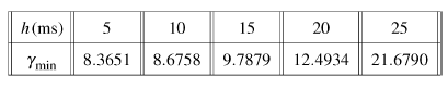
     5    10    15    20    25
gamma_min =
    8.3551    8.6451    9.7592   12.4787   21.6494

Below is the optimization result from Table II in the paper [1]:

% Plot the H_infinity gains
figure
plot(H.*1000,gamma_min,'k.','markersize',20)
xlabel('Max Sampling Interval [ms]')
ylabel('\gamma_{min}')
title('Guaranteed H_{\infty} Performance at Diff. Sampling Interals')

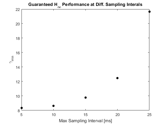
Fig. 2. $\gamma_{min}$ for different $h$ values.

% Simulation %%%%%%%%%%%%%%%%%%%%%%%%%%%%%%%%%%%%%%%%%%%%%%%%%%%%%%%%%%%%%%
h=10e-3;    % User specified max sampling time. The paper used 10ms
index=find(H==h);
K=K(index,:);   % find the optimal gains corresponding to the h value
dt=0.5e-3;   % simulated time step for continuous time
tEnd=5; % time horizon
% disturbance given in Equation (36)
a=0.06;
L=5;
V=45./3.6;  % speed in m/s
% Initialization of sampled-data system
x_S=zeros(4,1); % time history of states for sampled-data system
u_S=0;  % time history of input for sampled-data system
z1_S=[C1*x_S(:,end)];   % time history of output for sampled-data system
z2_S=[C2*x_S(:,end)];
% Initialization of passive system
xp_S=zeros(4,1); % time history of states for passive system
z1p_S=[C1*xp_S(:,end)]; % time history of output for passive system
z2p_S=[C2*xp_S(:,end)];
% Initilization of continuous-time system
xc_S=zeros(4,1); % time history of states for continuous-time system
% optimal feedback gain for continuous-time system, from Section IV
Kc=10e4*[-8.9220, -0.1447, -3.6650, 0.1494];
uc_S=0; % time history of input for continuous-time system
z1c_S=[C1*xc_S(:,end)]; % time history of output for continuous-time system
z2c_S=[C2*xc_S(:,end)];
t=0;    % starting time
% m is the maximum times of iteration where the input for the sampled-data
% system stays constant. m must be an integer.
m=h./dt;
iter_count=0;   % simulation iteration count
while t<tEnd
    temp=ceil(rand()*m);    % simulate un-uniform sampling period
    for counter=1:temp
        % current disturbance
        if t<=L./V
            w=pi.*a*V./L*sin(2*pi*V*t./L);
        else
            w=0;
        end
        % update passive system
        x=xp_S(:,end);  % current states
        xdot=A*x+B1*w;  % time derivative of states
        xp_S=[xp_S, x+xdot.*dt];    % update states
        z1p_S=[z1p_S, C1*xp_S(:,end)];   % update measurements
        z2p_S=[z2p_S, C2*xp_S(:,end)];
        % update continuous time system
        x=xc_S(:,end);  % current states
        u=Kc*x;  % calclate input
        xdot=A*x+B1*w+B*u;  % time derivative of states
        uc_S=[uc_S, u]; % record input data
        xc_S=[xc_S, x+xdot.*dt];    % update states
        z1c_S=[z1c_S, C1*xc_S(:,end)];   % update measurements
        z2c_S=[z2c_S, C2*xc_S(:,end)];
        % update sampled-data system
        x=x_S(:,end);   % current states
        if counter==1
            u=K*x;  % update input only at beginning of sampling period
        else
            u=u_S(end);     % otherwise use the previous input value
        end
        xdot=A*x+B1*w+B*u; % time derivative of states
        x_S=[x_S, x+xdot.*dt];  % update states and input
        u_S=[u_S, u];   % record input
        z1_S=[z1_S, C1*x_S(:,end)]; % update measurements
        z2_S=[z2_S, C2*x_S(:,end)];

        iter_count=iter_count+1;    % update iteration count
        t=dt.*iter_count;   % update current time
        if t>=tEnd   % break out of simulation when tEnd is reached
            break
        end
    end
end
% Plot Simulation Results %%%%%%%%%%%%%%%%%%%%%%%%%%%%%%%%%%%%%%%%%%%%%%%%%
% Note that the plot for hte sampled0data system may be slightly different
% from those in the paper because of the random sampling period.
i=0.025./dt;   % skip data for plotting to avoid clutter
t=0:dt:tEnd;
% Plot body acceleration
figure
plot(t(1:i:end),z1p_S(1:i:end),'m.',t(1:i:end),z1c_S(1:i:end),'b-.',...
    t(1:i:end),z1_S(1:i:end),'k-');
title('Body Acceleration [m/s^{2}]')
xlabel('Time [s]')
axis([0,5,-3,2])
legend('Passive','CT','Sampled')
% Plot suspension deflection
figure
plot(t(1:i:end),z2p_S(1,1:i:end),'m.',t(1:i:end),z2c_S(1,1:i:end),...
    'b-.',t(1:i:end),z2_S(1,1:i:end),'k-');
title('Suspension Deflection [m]')
xlabel('Time [s]')
axis([0,5,-0.05,0.05])
legend('Passive','CT','Sampled')
% Plot relative tyre load. Note the figure in the paper was labeled wrong.
% It should not be tyre deflection.
figure
plot(t(1:i:end),z2p_S(2,1:i:end),'m.',t(1:i:end),z2c_S(2,1:i:end),...
    'b-.',t(1:i:end),z2_S(2,1:i:end),'k-');
title('Relative Dynamic Tire Load')
xlabel('Time [s]')
axis([0,5,-0.2,0.2])
legend('Passive','CT','Sampled')
% Plot actuator input
figure
plot(t(1:i:end),uc_S(1:i:end),'b-.',t(1:i:end),u_S(1:i:end),'k-');
title('Actuator Input [N]')
xlabel('Time [s]')
axis([0,5,-2000,1500])
legend('CT','Sampled')

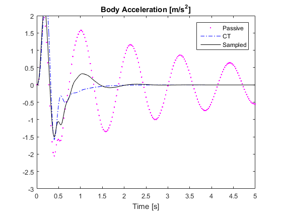
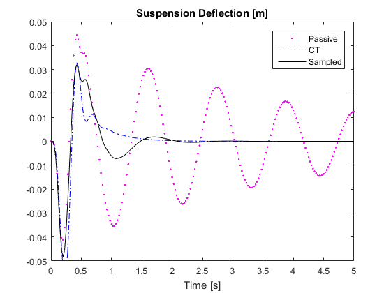
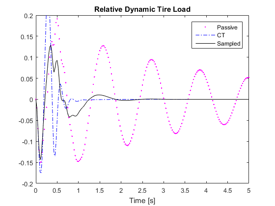
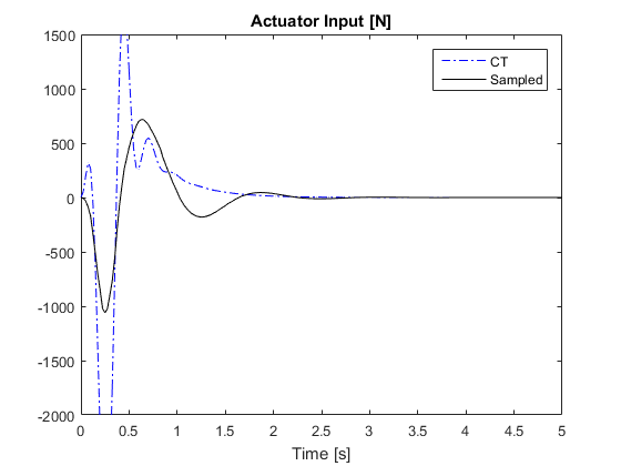
Fig. 3. Reproduction of the simulation result of the deterministic system.

Fig. 4. Simulation result given in the paper for the deterministic system [1].

6. Nondeterministic System Case

In this section, the uncertain system case is considered to verify the robustness of the sampled-data controller under suspension system uncertainties. For this specific example, it is assumed that the sprung mass and unsprung mass are uncertain within certain bounds. The performance of the controller is evaluated for each extreme case.

% The nominal system model is the same as the deterministic model.
% Lambdas give the uncertainties in the system parameters, in this case the
% sprung and unsprung mass. It defines a four-vertex polytopic system.
lambdas=[100, -100, 100, -100;
         10, 10, -10, -10];
% Optimization %%%%%%%%%%%%%%%%%%%%%%%%%%%%%%%%%%%%%%%%%%%%%%%%%%%%%%%%%%%%
cvx_begin quiet;
    variable Gamma2;    % Gamma.^2
    variable P_bar(4,4) symmetric;
    variable Q_bar(4,4) symmetric;
    % Note that there is a typo in the paper. S_bar is not a square
    % matrix and cannot be positive definite
    variable S_bar(9,4);
    variable K_bar(1,4);
    minimize (Gamma2)
    subject to
        % Gamma square should be non-negative
        Gamma2 >= 0;
        % P_bar and Q_bar are positive semi-definite
        P_bar == semidefinite(4);
        Q_bar == semidefinite(4);
        % The following constriants must be met at all 4 vertices
        for n=1:4
            % lambda and masses for the current vertex
            lambda1=lambdas(1,n); lambda2=lambdas(2,n);
            ms=973+lambda1;
            mu=114+lambda2;
            % System matrices for the current vertex
            A=[0,0,1,-1;
               0,0,0,1;
               -ks./ms,0,-cs./ms,cs./ms;
               ks./mu,-kt./mu,cs./mu,-(cs+ct)./mu];
            B=[0;0;1./ms;-1./mu];
            B1=[0;-1;0;ct./mu];
            C1=[-ks./ms,0,-cs./ms,cs./ms];
            D1=1./ms;
            C2=[1,0,0,0;
                0,kt./(ms+mu)./g,0,0];
            % Equation (34)
            Psi_bar1=[A*P_bar+P_bar*A.', B*K_bar, B1;
                  (B*K_bar).', zeros(4,4), zeros(4,1);
                  (B1).', zeros(1,4), zeros(1,1)];
            Psi_bar2=[S_bar, -S_bar, zeros(9,1)];
            Psi_5=-Gamma2.*eye(9);
            Psi_5(1:8,1:8)=zeros(8,8);
            Phi_bar1=[A*P_bar, B*K_bar, B1];
            Phi_bar2=[C1*P_bar, D1*K_bar, 0];
            % Equation (31)
            Mat1=[Psi_bar1+Psi_bar2+Psi_bar2.'+Psi_5, sqrt(h).*Phi_bar1.', ...
                        sqrt(h).*S_bar, Phi_bar2.';
                  sqrt(h).*Phi_bar1, Q_bar-2*P_bar, zeros(4,4), zeros(4,1);
                  sqrt(h).*S_bar.', zeros(4,4), -Q_bar, zeros(4,1);
                  Phi_bar2, zeros(1,4), zeros(1,4), -1];
            % Equation (32) for j=1
            Mat21=[-eye(1), sqrt(rho).*C2(1,:)*P_bar;
                  (sqrt(rho).*C2(1,:)*P_bar).', -z_max.^2*P_bar];
            % Equation (32) for j=2
            Mat22=[-eye(1), sqrt(rho).*C2(2,:)*P_bar;
                   (sqrt(rho).*C2(2,:)*P_bar).', -P_bar];
            % Equation (33)
            Mat3=[-eye(1), sqrt(rho).*K_bar;
                  (sqrt(rho).*K_bar).', -u_max.^2*P_bar];
            % Equation 31-33 are negative semi-definite, or the negative of
            % these matrices are positive semi-definite.
            0-Mat1 == semidefinite(18);
            0-Mat21 == semidefinite(5);
            0-Mat22 == semidefinite(5);
            0-Mat3 == semidefinite(5);
        end
cvx_end;
% Record the values of gamma and control gains
gamma_min=sqrt(Gamma2)
K=K_bar*inv(P_bar)
% Simulation %%%%%%%%%%%%%%%%%%%%%%%%%%%%%%%%%%%%%%%%%%%%%%%%%%%%%%%%%%%%%%
% disturbance given in Equation (36)
a=0.06;
L=5;
V=45./3.6;  % speed in m/s
% m is the maximum times of iteration where the input for the sampled-data
% system stays constant. m must be an integer.
m=h./dt;
legends={}; % place holder for plot legends
fig1=figure;
fig2=figure;
fig3=figure;
fig4=figure;
% Simulate for each vertex
for n=1:4
        % lambda and masses at the current vertex
        lambda1=lambdas(1,n); lambda2=lambdas(2,n);
        ms=973+lambda1;
        mu=114+lambda2;
        % system matrices at the current vertex
        A=[0,0,1,-1;
           0,0,0,1;
           -ks./ms,0,-cs./ms,cs./ms;
           ks./mu,-kt./mu,cs./mu,-(cs+ct)./mu];
        B=[0;0;1./ms;-1./mu];
        B1=[0;-1;0;ct./mu];
        C1=[-ks./ms,0,-cs./ms,cs./ms];
        D1=1./ms;
        C2=[1,0,0,0;
            0,kt./(ms+mu)./g,0,0];
        % initialization of sampled-data system
        x_S=zeros(4,1); % time history of states
        u_S=0;  % time history of input
        z1_S=[C1*x_S(:,end)];   % time history of measurements
        z2_S=[C2*x_S(:,end)];
        t=0; iter_count=0;      % starting time and iteration count
    while t<tEnd
        temp=ceil(rand()*m);    % simulate un-uniform sampling period
        for counter=1:temp
            % current disturbance
            if t<=L./V
                w=pi.*a*V./L*sin(2*pi*V*t./L);
            else
                w=0;
            end
            % update sampled-data system
            x=x_S(:,end);   % current states
            if counter==1
                u=K*x;  % update input only at beginning of sampling period
            else
                u=u_S(end);     % otherwise use the previous input value
            end
            xdot=A*x+B1*w+B*u;
            x_S=[x_S, x+xdot.*dt];  % update states and input
            u_S=[u_S, u];   % time derivative of states
            z1_S=[z1_S, C1*x_S(:,end)]; % update measurements
            z2_S=[z2_S, C2*x_S(:,end)];
            iter_count=iter_count+1;    % update iteration count and time
            t=dt.*iter_count;
            if t>=tEnd    % break out of simulation when tEnd is reached
                break
            end
        end
    end
    t=0:dt:tEnd;
    % update legend in each iteration
    legends{n}=['\lambda_{1}=',num2str(lambda1),' \lambda_{2}=' num2str(lambda2)];
    % Plot body acceleration
    figure(fig1); hold on; plot(t(:),z1_S(:));
    % Plot suspension deflection
    figure(fig2); hold on; plot(t(:),z2_S(1,:));
    % Plot relative tyre load. Note the figure in the paper was labeled wrong.
    % It should not be tyre deflection.
    figure(fig3); hold on; plot(t(:),z2_S(2,:));
    % Plot actuator input
    figure(fig4); hold on; plot(t(:),u_S(:));
end
% Add legends and labels, and format each figure.
figure(fig1);title('Body Acceleration [m/s^{2}]'); box on;
xlabel('Time [s]');axis([0,5,-3,3]);legend(legends);
figure(fig2);title('Suspension Deflection [m]'); box on;
xlabel('Time [s]');axis([0,5,-0.05,0.05]);legend(legends);
figure(fig3);title('Relative Dynamic Tire Load'); box on;
xlabel('Time [s]');axis([0,5,-0.2,0.2]);legend(legends);
figure(fig4);title('Actuator Input [N]'); box on;
xlabel('Time [s]');axis([0,5,-2000,1500]);legend(legends);

gamma_min =
   10.4150
K =
   1.0e+03 *
    1.2865    3.9585   -5.5926    0.5445

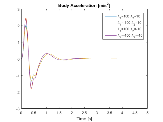
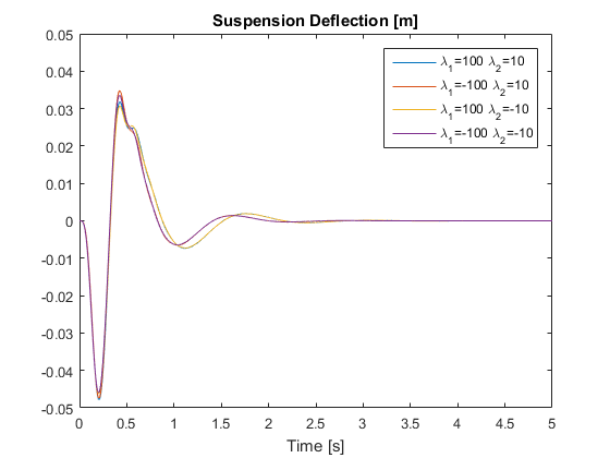
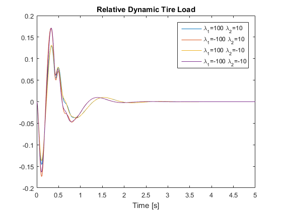
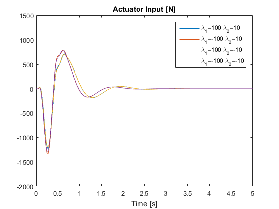
Fig. 5. Reproduction of the simulation result of the nondeterministic system.

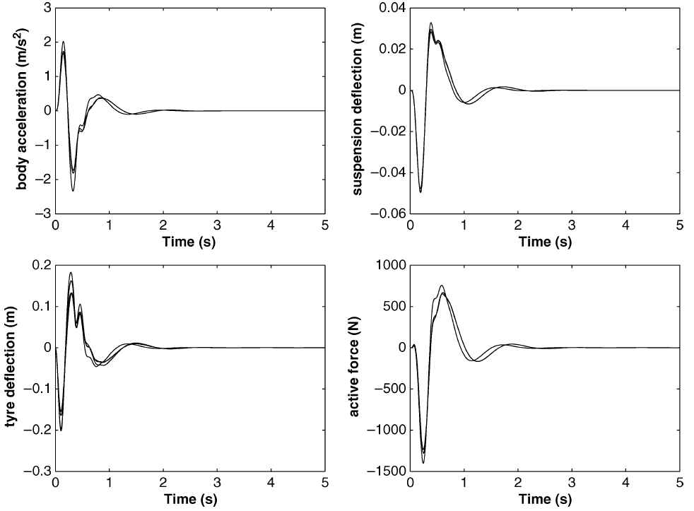
Fig. 6. Simulation result given in the paper for the nondeterministic system [1].

7. Analysis and Conclusions

The problem of robust sampled-data control for uncertain active vehicle suspension systems is reproduced. We were able to accurately reproduce the simulation results presented in the original paper using CVX [1-3]. Given information of quarter-car model parameters, the guaranteed $H_\infty$ performance $\gamma_{min}$ for different sampling intervals are obtained and all plots match very well with those in the original paper.
The algorithm and results supported those made by the authors. For the deterministic system, the responses of the passive system, the continuous-time closed-loop system and the sampled-data closed-loop system are simulated and compared. For the nondeterministic system, the robustness of the proposed controller is verified. In all cases, the 3 design objectives listed in Section 2 are met by the controller.
Drawbacks: 1) The system states are required to be measurable. When the state variables are unmeasurable or unknown, a dynamic output-feedback sampled-data controller is to be designed to improve the suspension performances, for instance, using the fuzzy model. 2) For the nondeterministic system, only the vertices of the polytopic system are considered for the constraints. It is not clear if these vertices are indeed the worst-case scenario. 3) Compuation for the optimal gains cannot happen in real-time because of the complexity of the algorithm. 4) The constraints for the optimization give a sufficient condition for the existance of a controller that satisfies the design objective, but they may not be necessary.

8. References

[1] Gao H, Sun W, Shi P. Robust Sampled-Data $H_\infty$ Control for Vehicle Active Suspension Systems. IEEE Transactions on Control Systems Technology. 2010 Jan;18(1):238-45.

[2] Boyd, Stephen, and Lieven Vandenberghe. Convex Optimization. Cambridge University Press, 2004.

[3] Grant, Michael, Stephen Boyd, and Yinyu Ye. "CVX: Matlab Software for Disciplined Convex Programming," 2008.

[4] H. Du and N. Zhang, $H_\infty$ control of active vehicle suspensions with actuator time delay, J. Sound Vib., vol. 301, pp. 236?52, 2007.