Estimation of Faults in DC Electrical Power Systems.

. Student names: Ahmed Abdalrahman Ahmed and Farid Farmani .

Course: ECE 602- Winter 2017

Introduction
Problem description
System model
Data sources
Simulation study
Visualization of results
Conclusion
Reference

Introduction

. The goal of this project is to replicate and analyze the estimation methods provided in [1]. It is noteworthy to say that the results provided in [1] was experimentally achieved, and do to lack of equipment we solely focus on simulation studies.

Problem description

. The main goal of this paper is to estimate faults in a DC electric circuit via optimization methods. A DC electric circuit consists of sources, loads and switching elements. voltage and current measurements are implemented on some specific nodes in the system. The problem is how to use these measurements to estimate the fault states of the circuit. In this paper a circuit model of the form:

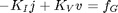
Is considered to estimate faults $f$ , in which matrices A, B, C, D have appropriate dimensions. Indeed, the problem is to estimate faults f given the vector of observations y. The process noise vector ${\xi}$ describes the modelling error, and the measurement noise ${\eta}$ describes the observation error.

The faults $f$ and the states $x$ are estimated by solving a quadratic programming (QP) problem of the form:

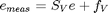
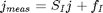
Where $\|z\|^2_Q=z^TQz$ ; Q, R are positive definite matrices; $|f|$ is the component-wise absolute value; $\lambda$ is a vector with positive components. The last term provides a weighted $l_1$ penalty for the unknown components of vector $f$ .

The problem is solved using standard QP software.

System model

. The problem formulation consists of three parts which are discussed as follows.

I) State equations

. The STA equations of the DC nodal are formulated in a standard way. STA models are the core of most standard small-signal liear analysis of electric circuits.

The circuit has nodes; each node has a voltage with respect to the ground
The circuit contains branches, each has current and voltage drop .
The signs of the currents and the voltage drops are relative to the directions of respective branches (graph edges).
The incidence matrix $G \in \Re^{N_N,N_B}$ has entries $g_{kl}$ =1 if the branch leaves the node , $g_{kl}$ = -1 if it enters node , and $g_{kl}$ = 0 otherwise.
The STA equations comprise , and .

. The KCL equations for the currents are

$${S_B}{G_j}=0$

. The KVL relates voltage drops v to the node voltages $e

$${G^T}{e}=v$

. Finally the BCE relates the voltage drop and the current.

$$-K_I{j}+K_V{v}=f_G$

. Three types of faults are considered in this study:

1) The fault of switching element k, which is thought open but might be actually closed.

$$-j_k=f_{G,k}$

2) The fault of a switching element k, which is thought closed.

$v_k=f_{G,k}$

3) The fault of the DC load.

$g_k{v_k}-j_k=f_{G,k}$

II) Observation equations

. The observation equations regarding the currents measured by current sensors and voltages measured by voltages sensors have the form.

$e_{meas}=S_V{e}+f_V$

$j_{meas}=S_I{j}+f_I$

. The observation equations regarding the known voltage sources and grounded nodes have the form:

$e_{srce}=S_S{e}+f_S$

$e_{grnd}=S_{G}e$

III) STA MODEL with faults

In order to obtain a linear model of the form (1) and (2) we define.

The noises are considered to be zero in this study. These matrices are all used to solve the optimization problem (3) to estimate the faults.

Data sources

The ADAPT circuit which is shown in Figure 1 is used for simulation studies [1].

. The authors specified the problem parameters in the paper. We used identical parameters in our simulations. These parameters are defined here.

Simulation study

. The following code is written to solve the estimation problem. In this part the state and observation equations as well as STA model (which were previously discussed) is provided.

-State equations:

clc
clear

% The incidence matrix G
G = zeros (18,18);

G(1,1)= 1;  G(2,1)=-1;   G(2,2)=1;  G(3,2)=-1; G(3,3)=1;
G(4,3)=-1;  G(4,4)=-1;   G(12,4)=1; G(4,5)=1;  G(5,5)=-1;
G(5,6)=1;   G(6,6)=-1;   G(6,7)=1;  G(7,7)=-1;
G(5,8)=1;   G(8,8)=-1;   G(8,9)=1;  G(9,9)=-1;

G(10,10)=1;  G(11,10)=-1; G(11,11)=1;  G(12,11)=-1; G(12,12)=1;
G(13,12)=-1; G(3,13)=1;   G(13,13)=-1; G(13,14)=1;  G(14,14)=-1;
G(14,15)=1;  G(15,15)=-1; G(15,16)=1;  G(16,16)=-1; G(14,17)=1;
G(17,17)=-1; G(17,18)=1;  G(18,18)=-1;

% The selection matrix SB that un-selects the boundary nodes of the circuit
% where KCL does not hold.
SB= ones (18,18);

SB(1,1)=0; SB(10,10)=0; SB(9,9)=0; SB(7,7)=0; SB(16,16)=0; SB(18,18)=0;

% Ki (Diagonal Matrix) diagonal entry of KI could be a branch resistance
%branch resistans
Res= [0.1 0 10^15 0 0 0 6 0 10 0.1 0 0 10^15 0 0 4 0 20];
Ki = diag (Res);

% Kv unity Diagonal Matrix
Kv = eye(18);

% The Branches current vector J
J=  sym('J', [18 1]);

% Voltage drop on Branches vector V
V= sym('V', [18 1]);

% Nodal volatage vector E
E= sym('e', [18 1]);

%The KCL equations for the currents j
kcl= zeros (18,1);
% disp( sprintf( 'KCL Equations'));
SB.*G*J == kcl;

%The KVL relates voltage drops V  to the node voltages E
% disp( sprintf( 'KVL Equations '));
G.'*E == V;

%Branch Constitutive Equations (BCE)
Fg = sym('Fg', [18 1]);
% disp( sprintf( 'Branch Constitutive Equations (BCE)'));
- Ki*J + Kv*V == Fg;

%

-Observation equations

Jms = sym('Jms', [18 1]);  % current sensors
Ems = sym('Ems', [18 1]); % Volatage sensors

Esrc = zeros (18,1); %  Voltage sources
Esrc(1,1)= 25.48;  Esrc(10,1)=24.83;

Egrd = zeros (18,1); %  ground nodes
Egrd(7,1)= 0;  Egrd(9,1)= 0;  Egrd(16,1)=0;  Egrd(18,1)=0;

Fs = sym('Fs', [18 1]); % Fault offsets in voltage source
FV = sym('FV', [18 1]); % Fault offsets in voltage sensor
FI = sym('FI', [18 1]); % Fault offsets in Current sensor

SI = zeros (18,18); %  selection matrices for branches with current sensor
SI(1,1)= 1;  SI(5,5)= 1; SI(8,8)= 1;
SI(10,10)=1;  SI(14,14)=1; SI(17,17)=1;

SV = zeros (18,18); %  selection matrices for nodes with voltage sensor
SV(2,2)=1;   SV(3,3)=1;  SV(4,4)=1;  SV(5,5)=1; SV(8,8)=1;
SV(11,11)=1;  SV(12,12)=1; SV(13,13)=1; SV(14,14)=1; SV(17,17)=1;

Ss = zeros (18,18); %  selection matrices voltage sources
Ss(1,1)= 1;  Ss(10,10)= 1;

Sg = zeros (18,18); %  selection matrices ground nodes
Sg(7,7)= 1;  Sg(9,9)= 1;  Sg(16,16)=1;  Sg(18,18)=1;

SV*Ems == SV*E + SV*FV;
SI*Jms == SI*J + FI;

Esrc == Ss*E + Fs;
Egrd == Sg*E;

-STA model

A = [SB.*G,       zeros(18,18), zeros(18,18); ...
    zeros(18,18),  eye(18),        -G.'     ; ...
    Ki,              Kv,         zeros(18,18)];

X = [J;V;E];

F= [Fg; FI; FV; Fs];

B= [zeros(36,72); eye(18), zeros(18,54)];

% Y = [Jms;Ems;Esrc;Egrd];      % when faults are considered
Y = [zeros(36,1);Esrc;Egrd];    % no faults assumption


% C = [SI, zeros(18,36); ...    % when faults are considered
%     zeros(18,36), SV; ...
%     zeros(18,36), Ss; ...
%     zeros(18,36), Sg];

C = [ zeros(36,54); ...         % no faults assumption
    zeros(18,36), Ss; ...
    zeros(18,36), Sg];

% D = [zeros(18,18), SI, zeros(18,36); ...  % when faults are considered
%     zeros(18,36), SV, zeros(18,18); ...
%     zeros(18,54), Ss; zeros(18,72)];

D = [ zeros(36,72); ...        % no faults assumption
    zeros(18,54), Ss; zeros(18,72)];

% disp( sprintf( 'Circuit analysis equations '));
% A*X + B*F == 0              % Model equations
% Y == C*X + D*F

Visualization of results

The optimization problem (3) is solved to obtain the estimation of faults. two case studies are considered for this reason. These include base case with no faults in the system and two other cases with multiple faults in the system.

. Case (1): base case, no faults occurred

. In this case we only calculate the true states of the circuit based on its parameters. Indeed, wrong data from sensors is ignored in this case.

cvx_begin
variables XX(54,1) FF(72,1)
minimize  0.5 * (square_pos(norm((A*XX + B*FF),2)) + square_pos(norm((C*XX+D*FF - Y),2)))+ norm(FF,1)
cvx_end

% Display Results
JJ = XX(1:18,1);
VV = XX(19:36,1);
EE = XX(37:54,1);
FFg = FF(1:18,1);
FFI = FF(19:36,1);
FFV = FF(37:54,1);
FFs = FF(55:72,1);
disp( sprintf( '\nResults: Without any Faults\n=========================\ncvx_optval: %6.4f\ncvx_status: %s\n',cvx_optval, cvx_status ) );
disp( ['Branches Currents (A)'] );
disp( [ '   J  = [ ', sprintf( '%7.4f ', JJ.'), ']'] );
disp( [ sprintf( '\n'),'Branches Voltages (V)' ] );
disp( [ '   V  = [ ', sprintf( '%7.4f ', VV.'), ']'] );
disp( [ sprintf( '\n'),'Node Voltages (V)' ] );
disp( [ '   E  = [ ', sprintf( '%7.4f ', EE.'), ']'] );
disp( [sprintf( '\n'),'Faults in the branches'] );
disp( [ '   Fg  = [ ', sprintf( '%7.4f ', FFg.'), ']'] );
disp( [sprintf( '\n'), 'Fault offsets in Current' ] );
disp( [ '   Fi  = [ ', sprintf( '%7.4f ', FFI.'), ']'] );
disp( [ sprintf( '\n'),'Fault offsets in Voltages' ] );
disp( [ '   Fv  = [ ', sprintf( '%7.4f ', FFV.'), ']'] );
disp( [ sprintf( '\n'),'Fault offsets in Sources' ] );
disp( [ '   Fs  = [ ', sprintf( '%7.4f ', FFs.'), ']'] );

 
Calling SDPT3 4.0: 210 variables, 4 equality constraints
------------------------------------------------------------

 num. of constraints =  4
 dim. of sdp    var  =  4,   num. of sdp  blk  =  2
 dim. of socp   var  = 200,   num. of socp blk  = 74
 dim. of linear var  =  4
*******************************************************************
   SDPT3: Infeasible path-following algorithms
*******************************************************************
 version  predcorr  gam  expon  scale_data
   HKM      1      0.000   1        0    
it pstep dstep pinfeas dinfeas  gap      prim-obj      dual-obj    cputime
-------------------------------------------------------------------
 0|0.000|0.000|1.8e+01|8.2e+00|2.9e+03| 2.136468e+02  0.000000e+00| 0:0:00| chol  1  1 
 1|0.943|0.914|1.1e+00|8.0e-01|3.9e+02| 1.737205e+02 -1.782110e+01| 0:0:00| chol  1  1 
 2|1.000|1.000|1.9e-06|9.5e-03|4.8e+01| 4.122156e+01 -5.731491e+00| 0:0:00| chol  1  1 
 3|0.769|0.869|7.7e-07|2.1e-03|1.7e+01| 1.500651e+01 -1.623734e+00| 0:0:00| chol  1  1 
 4|0.784|0.884|2.7e-07|3.2e-04|6.4e+00| 5.926317e+00 -4.264537e-01| 0:0:00| chol  1  1 
 5|0.793|0.849|5.8e-08|5.7e-05|2.3e+00| 2.170577e+00 -1.638404e-01| 0:0:00| chol  1  1 
 6|0.771|0.900|1.4e-08|6.6e-06|8.6e-01| 8.034017e-01 -5.328292e-02| 0:0:00| chol  1  1 
 7|0.973|0.911|1.0e-09|6.7e-07|1.8e-01| 1.686089e-01 -1.254945e-02| 0:0:00| chol  1  1 
 8|0.879|0.922|3.4e-10|6.1e-08|4.0e-02| 3.777079e-02 -2.575053e-03| 0:0:00| chol  1  1 
 9|0.955|0.904|2.6e-10|6.8e-09|8.4e-03| 7.801219e-03 -5.766698e-04| 0:0:00| chol  1  1 
10|0.849|0.907|3.9e-11|7.7e-10|2.1e-03| 1.992721e-03 -1.349146e-04| 0:0:00| chol  1  1 
11|0.933|0.894|2.6e-12|9.8e-11|5.0e-04| 4.644292e-04 -3.330480e-05| 0:0:00| chol  1  1 
12|0.861|0.917|3.6e-13|1.0e-11|1.3e-04| 1.205087e-04 -8.029342e-06| 0:0:00| chol  1  1 
13|0.940|0.906|2.2e-14|2.0e-12|2.9e-05| 2.681777e-05 -1.904394e-06| 0:0:00| chol  1  1 
14|0.882|0.930|2.6e-15|1.1e-12|7.2e-06| 6.715195e-06 -4.437531e-07| 0:0:00| chol  1  1 
15|0.934|0.912|2.1e-16|1.1e-12|1.6e-06| 1.484704e-06 -1.039534e-07| 0:0:00| chol  1  1 
16|0.886|0.930|9.4e-17|1.1e-12|3.9e-07| 3.674896e-07 -2.401884e-08| 0:0:00| chol  1  1 
17|0.587|0.931|2.1e-16|1.1e-12|2.0e-07| 1.943996e-07 -6.006972e-09| 0:0:00| chol  1  1 
18|0.587|1.000|9.2e-17|1.0e-12|1.1e-07| 1.024017e-07 -3.357546e-09| 0:0:00| chol  1  1 
19|0.586|1.000|1.3e-16|1.0e-12|5.6e-08| 5.412116e-08 -1.518145e-09| 0:0:00| chol  1  1 
20|0.585|1.000|1.8e-16|1.0e-12|2.9e-08| 2.861506e-08 -7.825540e-10| 0:0:00| chol  1  1 
21|0.585|1.000|9.2e-17|1.0e-12|1.6e-08| 1.513174e-08 -4.077402e-10| 0:0:00| chol  1  1 
22|0.585|1.000|1.0e-16|1.0e-12|8.2e-09| 8.001494e-09 -2.145746e-10| 0:0:00|
  stop: max(relative gap, infeasibilities) < 1.49e-08
-------------------------------------------------------------------
 number of iterations   = 22
 primal objective value =  8.00149415e-09
 dual   objective value = -2.14574646e-10
 gap := trace(XZ)       = 8.22e-09
 relative gap           = 8.22e-09
 actual relative gap    = 8.22e-09
 rel. primal infeas (scaled problem)   = 1.03e-16
 rel. dual     "        "       "      = 1.00e-12
 rel. primal infeas (unscaled problem) = 0.00e+00
 rel. dual     "        "       "      = 0.00e+00
 norm(X), norm(y), norm(Z) = 1.4e+00, 1.5e-05, 8.5e+00
 norm(A), norm(b), norm(C) = 4.0e+00, 2.4e+00, 9.5e+00
 Total CPU time (secs)  = 0.33  
 CPU time per iteration = 0.01  
 termination code       =  0
 DIMACS: 1.2e-16  0.0e+00  4.8e-12  0.0e+00  8.2e-09  8.2e-09
-------------------------------------------------------------------
 
------------------------------------------------------------
Status: Solved
Optimal value (cvx_optval): +8.00149e-09
 

Results: Without any Faults
=========================
cvx_optval: 0.0000
cvx_status: Solved

Branches Currents (A)
   J  = [ -0.0000 -0.0000 -0.0000 -6.2662 -6.2662 -3.9164 -3.9164 -2.3498 -2.3498 -13.3158 -13.3158 -7.0495 -0.0000 -7.0495 -5.8746 -5.8746 -1.1749 -1.1749 ]

Branches Voltages (V)
   V  = [  0.0000  0.0000  1.9816  0.0000  0.0000  0.0000 23.4984  0.0000 23.4984  1.3316  0.0000  0.0000  1.9816  0.0000  0.0000 23.4984  0.0000 23.4984 ]

Node Voltages (V)
   E  = [ 25.4800 25.4800 25.4800 23.4984 23.4984 23.4984  0.0000 23.4984  0.0000 24.8300 23.4984 23.4984 23.4984 23.4984 23.4984  0.0000 23.4984  0.0000 ]

Faults in the branches
   Fg  = [  0.0000  0.0000  0.0000  0.0000  0.0000  0.0000  0.0000  0.0000  0.0000  0.0000  0.0000  0.0000  0.0000  0.0000  0.0000  0.0000  0.0000  0.0000 ]

Fault offsets in Current
   Fi  = [  0.0000  0.0000  0.0000  0.0000  0.0000  0.0000  0.0000  0.0000  0.0000  0.0000  0.0000  0.0000  0.0000  0.0000  0.0000  0.0000  0.0000  0.0000 ]

Fault offsets in Voltages
   Fv  = [  0.0000  0.0000  0.0000  0.0000  0.0000  0.0000  0.0000  0.0000  0.0000  0.0000  0.0000  0.0000  0.0000  0.0000  0.0000  0.0000  0.0000  0.0000 ]

Fault offsets in Sources
   Fs  = [  0.0000  0.0000  0.0000  0.0000  0.0000  0.0000  0.0000  0.0000  0.0000  0.0000  0.0000  0.0000  0.0000  0.0000  0.0000  0.0000  0.0000  0.0000 ]

Case (2): Optimization Problem with multiple faults in CB ISH280 and CS IT280

In this case, we assume ISH280 fails to operate properly (opens) and current sensor IT280 continues to show that it is closed. From the results, it can be seen that the model accurately estimate the faulted component and the value of the fault. In this case, the fault was in current sensor IT280 by (-0.1749 A), which is estimated in the Fault offsets in Current vector correctly.

KiErr =Ki;
KiErr(17,17)= 10^15; % circuit breaker resistance become Inf
Y3 = [JJ;EE;Esrc;Egrd]; % Sensors reading still as normal

AErr = [SB.*G,       zeros(18,18), zeros(18,18); ...  % when faults in CB is considered
    zeros(18,18),  eye(18),        -G.'     ; ...
    KiErr,              Kv,         zeros(18,18)];

C = [SI, zeros(18,36); ...   % when faults are considered
    zeros(18,36), SV; ...
    zeros(18,36), Ss; ...
    zeros(18,36), Sg];

D = [zeros(18,18), SI, zeros(18,36); ... % when faults are considered
    zeros(18,36), SV, zeros(18,18); ...
    zeros(18,54), Ss; zeros(18,72)];

cvx_begin
variables XX3(54,1) FF3(72,1)
minimize  0.5 * (square_pos(norm((AErr*XX3 + B*FF3),2)) + square_pos(norm((C*XX3+D*FF3 - Y3),2)))+ norm(FF3,1)
cvx_end

% Display Results
JJ3 = XX3(1:18,1);
VV3 = XX3(19:36,1);
EE3 = XX3(37:54,1);
FFg3 = FF3(1:18,1);
FFI3 = FF3(19:36,1);
FFV3 = FF3(37:54,1);
FFs3 = FF3(55:72,1);
disp( sprintf( '\n\nResults: With Faults in CB ISH280 and CS IT280' ) );
disp( sprintf( 'ISH280 fails (opens) and current sensor IT280 continues to show that it is closed.') );
disp( ['=========================================================='] );
disp( ['Branches Currents (A)'] );
disp( [ '   J  = [ ', sprintf( '%7.4f ', JJ3.'), ']'] );
disp( [ sprintf( '\n'),'Branches Voltages (V)' ] );
disp( [ '   V  = [ ', sprintf( '%7.4f ', VV3.'), ']'] );
disp( [ sprintf( '\n'),'Node Voltages (V)' ] );
disp( [ '   E  = [ ', sprintf( '%7.4f ', EE3.'), ']'] );
disp( [sprintf( '\n'),'Faults in the branches'] );
disp( [ '   Fg  = [ ', sprintf( '%7.4f ', FFg3.'), ']'] );
disp( [sprintf( '\n'), 'Fault offsets in Current' ] );
disp( [ '   Fi  = [ ', sprintf( '%7.4f ', FFI3.'), ']'] );
disp( [ sprintf( '\n'),'Fault offsets in Voltages' ] );
disp( [ '   Fv  = [ ', sprintf( '%7.4f ', FFV3.'), ']'] );
disp( [ sprintf( '\n'),'Fault offsets in Sources' ] );
disp( [ '   Fs  = [ ', sprintf( '%7.4f ', FFs3.'), ']'] );

 
Calling SDPT3 4.0: 229 variables, 23 equality constraints
------------------------------------------------------------

 num. of constraints = 23
 dim. of sdp    var  =  4,   num. of sdp  blk  =  2
 dim. of socp   var  = 217,   num. of socp blk  = 74
 dim. of linear var  =  4
 dim. of free   var  =  2 *** convert ublk to lblk
 number of nearly dependent constraints = 21
 To remove these constraints, re-run sqlp.m with OPTIONS.rmdepconstr = 1.
*******************************************************************
   SDPT3: Infeasible path-following algorithms
*******************************************************************
 version  predcorr  gam  expon  scale_data
   HKM      1      0.000   1        0    
it pstep dstep pinfeas dinfeas  gap      prim-obj      dual-obj    cputime
-------------------------------------------------------------------
 0|0.000|0.000|2.8e+05|1.4e+15|5.3e+31| 2.349842e+15  0.000000e+00| 0:0:00| chol  2 * 2 
 1|0.000|0.000|2.8e+05|1.4e+15|1.1e+31| 1.873243e+16 -8.920868e+01| 0:0:00| chol * 3 * 4 
 2|0.000|0.000|2.8e+05|1.4e+15|2.1e+30| 2.571843e+17 -2.321848e+03| 0:0:00| chol * 4 * 4 
 3|0.000|0.000|2.8e+05|1.4e+15|4.3e+29| 2.445826e+18 -1.994263e+04| 0:0:00| chol * 3 * 3 
 4|0.000|0.000|2.8e+05|1.4e+15|8.5e+28| 2.112631e+19 -1.850344e+05| 0:0:00|
 *** Too many tiny steps:  restarting with the following iterate.
 *** [X,y,Z] = infeaspt(blk,At,C,b,2,1e5); chol * 1  2 
 5|0.871|0.871|1.3e-01|1.3e+04|1.1e+11| 7.473886e+06 -2.064971e+05| 0:0:00| chol  2  2 
 6|0.691|0.691|4.0e-02|3.9e+03|3.8e+10| 8.437410e+06 -3.599287e+05| 0:0:00| chol  2  2 
 7|0.634|0.634|1.5e-02|1.4e+03|1.6e+10| 9.707247e+06 -5.045203e+05| 0:0:00| chol  2  2 
 8|0.627|0.627|5.4e-03|5.3e+02|6.7e+09| 1.118625e+07 -6.459437e+05| 0:0:00| chol  2  2 
 9|0.627|0.627|2.0e-03|2.0e+02|2.9e+09| 1.286652e+07 -7.881936e+05| 0:0:00| chol  2  2 
10|0.629|0.629|7.5e-04|7.3e+01|1.2e+09| 1.474331e+07 -9.344231e+05| 0:0:00| chol  2  2 
11|0.634|0.633|2.8e-04|2.7e+01|5.3e+08| 1.674703e+07 -1.082734e+06| 0:0:00| chol  2  2 
12|0.648|0.647|9.7e-05|9.5e+00|2.2e+08| 1.859116e+07 -1.215759e+06| 0:0:00| chol  2  2 
13|0.691|0.686|3.0e-05|3.0e+00|8.6e+07| 1.931836e+07 -1.269804e+06| 0:0:00| chol  2  2 
14|0.878|0.842|3.7e-06|4.7e-01|2.5e+07| 1.557062e+07 -1.027706e+06| 0:0:00| chol  2  2 
15|0.690|0.656|1.1e-06|1.6e-01|7.8e+06| 6.253620e+06 -3.932139e+05| 0:0:00| chol  2  2 
16|0.613|0.680|4.4e-07|5.2e-02|4.1e+06| 3.542443e+06 -2.982110e+05| 0:0:00| chol  2  2 
17|1.000|0.190|2.2e-10|4.3e-02|1.1e+06| 8.110512e+05 -2.435122e+05| 0:0:00| chol  2  2 
18|1.000|0.751|3.7e-11|1.1e-02|2.3e+05| 1.818279e+05 -4.927174e+04| 0:0:00| chol  2  2 
19|0.874|0.747|1.8e-11|2.8e-03|4.9e+04| 3.929272e+04 -9.676952e+03| 0:0:00| chol  2  2 
20|0.937|0.324|1.6e-11|1.9e-03|1.8e+04| 1.157267e+04 -5.880880e+03| 0:0:01| chol  2  2 
21|1.000|0.474|1.6e-11|9.9e-04|6.5e+03| 4.173266e+03 -2.327447e+03| 0:0:01| chol  2  2 
22|0.995|0.534|6.1e-12|4.6e-04|2.5e+03| 2.137324e+03 -3.218428e+02| 0:0:01| chol  2  2 
23|0.952|0.474|1.9e-10|2.4e-04|1.2e+03| 1.640188e+03  4.900442e+02| 0:0:01| chol * 2  2 
24|0.963|0.432|2.1e-10|1.4e-04|6.0e+02| 1.473825e+03  8.743816e+02| 0:0:01| chol * 2 * 2 
25|1.000|0.423|2.7e-11|7.9e-05|3.3e+02| 1.412474e+03  1.086400e+03| 0:0:01| chol  2 * 2 
26|1.000|0.425|2.3e-10|4.6e-05|1.8e+02| 1.389885e+03  1.208756e+03| 0:0:01| chol * 2 * 2 
27|1.000|0.489|1.6e-10|2.3e-05|9.0e+01| 1.378795e+03  1.289296e+03| 0:0:01| chol * 2 * 2 
28|1.000|0.445|6.0e-11|1.3e-05|4.9e+01| 1.375199e+03  1.326683e+03| 0:0:01| chol * 2 * 2 
29|1.000|0.692|1.6e-10|4.0e-06|1.5e+01| 1.373380e+03  1.358817e+03| 0:0:01| chol * 2  2 
30|1.000|0.772|1.9e-11|9.0e-07|3.3e+00| 1.373088e+03  1.369825e+03| 0:0:01| chol  2  2 
31|0.975|0.884|1.5e-11|1.0e-07|3.8e-01| 1.373066e+03  1.372690e+03| 0:0:01| chol  2  2 
32|1.000|0.400|1.3e-12|6.3e-08|2.3e-01| 1.373065e+03  1.372840e+03| 0:0:01| chol * 2 * 2 
33|1.000|0.381|2.7e-12|3.9e-08|1.4e-01| 1.373065e+03  1.372926e+03| 0:0:01| chol * 2 * 2 
34|1.000|0.491|5.5e-12|2.0e-08|7.1e-02| 1.373065e+03  1.372994e+03| 0:0:01| chol * 2 * 2 
35|1.000|0.534|4.9e-12|9.2e-09|3.3e-02| 1.373065e+03  1.373032e+03| 0:0:01| chol * 2 * 2 
36|1.000|0.455|3.6e-13|5.0e-09|1.8e-02| 1.373065e+03  1.373047e+03| 0:0:01| chol * 2 * 2 
37|1.000|0.265|2.7e-12|5.4e-06|1.3e-02| 1.373065e+03  1.373052e+03| 0:0:01| chol  2  2 
38|1.000|0.983|2.9e-16|5.5e-06|2.9e-04| 1.373065e+03  1.373065e+03| 0:0:01| chol * 2 * 2 
39|0.989|0.989|6.4e-16|1.2e-07|3.3e-06| 1.373065e+03  1.373065e+03| 0:0:01| chol * 2 * 2 
40|0.727|0.944|4.3e-16|1.4e-09|1.9e-07| 1.373065e+03  1.373065e+03| 0:0:01|
  stop: max(relative gap, infeasibilities) < 1.49e-08
-------------------------------------------------------------------
 number of iterations   = 40
 primal objective value =  1.37306493e+03
 dual   objective value =  1.37306493e+03
 gap := trace(XZ)       = 1.89e-07
 relative gap           = 6.89e-11
 actual relative gap    = 6.51e-11
 rel. primal infeas (scaled problem)   = 4.26e-16
 rel. dual     "        "       "      = 1.39e-09
 rel. primal infeas (unscaled problem) = 0.00e+00
 rel. dual     "        "       "      = 0.00e+00
 norm(X), norm(y), norm(Z) = 2.7e+03, 1.4e+03, 1.4e+03
 norm(A), norm(b), norm(C) = 2.0e+15, 1.2e+15, 9.5e+00
 Total CPU time (secs)  = 0.94  
 CPU time per iteration = 0.02  
 termination code       =  0
 DIMACS: 4.3e-16  0.0e+00  6.6e-09  0.0e+00  6.5e-11  6.9e-11
-------------------------------------------------------------------
 
------------------------------------------------------------
Status: Solved
Optimal value (cvx_optval): +1373.06
 


Results: With Faults in CB ISH280 and CS IT280
ISH280 fails (opens) and current sensor IT280 continues to show that it is closed.
==========================================================
Branches Currents (A)
   J  = [  0.0000  0.0000 -0.0000 -6.3603 -6.3059 -3.9336 -3.9188 -2.3574 -2.3502 -13.2615 -13.2070 -6.7923 -0.0000 -6.7379 -6.3718 -6.0057  0.0000 -1.1633 ]

Branches Voltages (V)
   V  = [ -0.0000 -0.0000  1.9800  0.0014 -0.0002 -0.0025 23.5102  0.0004 23.5010  1.3272 -0.0011 -0.0068  1.9638 -0.0246 -0.0915 23.9314  0.1251 23.3239 ]

Node Voltages (V)
   E  = [ 25.4800 25.4800 25.4800 23.5000 23.5003 23.5053 -0.0025 23.4995 -0.0007 24.8289 23.5006 23.5027 23.5162 23.5654 23.7484 -0.0915 23.4403  0.0582 ]

Faults in the branches
   Fg  = [  0.0000  0.0000 -0.0000 -0.0000  0.0000  0.0000  0.0000 -0.0000  0.0000 -0.0000  0.0000  0.0000 -0.0000  0.0000  0.0000  0.0000  0.0000 -0.0000 ]

Fault offsets in Current
   Fi  = [ -0.0000  0.0000  0.0000  0.0000  0.0000  0.0000  0.0000  0.0000  0.0000 -0.0000  0.0000  0.0000  0.0000 -0.0000  0.0000  0.0000 -0.1749  0.0000 ]

Fault offsets in Voltages
   Fv  = [  0.0000 -0.0000 -0.0000 -0.0000 -0.0000  0.0000  0.0000 -0.0000  0.0000  0.0000 -0.0000 -0.0000 -0.0000 -0.0000  0.0000  0.0000  0.0000  0.0000 ]

Fault offsets in Sources
   Fs  = [ -0.0000  0.0000  0.0000  0.0000  0.0000  0.0000  0.0000  0.0000  0.0000  0.0000  0.0000  0.0000  0.0000  0.0000  0.0000  0.0000  0.0000  0.0000 ]

Case (3): Optimization Problem with multiple faults in CB ISH180 and CS IT180

In this case, we assume ISH180 fails to operate properly (opens) and current sensor IT180 continues to show that it is closed. From the results, it can be seen that the model accurately estimate the faulted component and the value of the fault. In this case, the fault was in current sensor IT180 by (-1.3499 A), which is estimated in the Fault offsets in Current vector correctly.

KiErr =Ki;
KiErr(8,8)= 10^15; % circuit breaker resistance become Inf
Y5 = [JJ;EE;Esrc;Egrd]; % Sensors reading still as normal

AErr = [SB.*G,       zeros(18,18), zeros(18,18); ...  % when faults in CB is considered
    zeros(18,18),  eye(18),        -G.'     ; ...
    KiErr,              Kv,         zeros(18,18)];

cvx_begin
variables XX5(54,1) FF5(72,1)
minimize  0.5 * (square_pos(norm((AErr*XX5 + B*FF5),2)) + square_pos(norm((C*XX5+D*FF5 - Y5),2)))+ norm(FF5,1)
cvx_end

% Display Results
JJ5 = XX5(1:18,1);
VV5 = XX5(19:36,1);
EE5 = XX5(37:54,1);
FFg5 = FF5(1:18,1);
FFI5 = FF5(19:36,1);
FFV5 = FF5(37:54,1);
FFs5 = FF5(55:72,1);
disp( sprintf( '\n\nResults: With Faults in CB ISH180 and CS IT180' ) );
disp( sprintf( 'ISH180 fails (opens) and current sensor IT180 continues to show that it is closed.') );
disp( ['=========================================================='] );
disp( ['Branches Currents (A)'] );
disp( [ '   J  = [ ', sprintf( '%7.4f ', JJ5.'), ']'] );
disp( [ sprintf( '\n'),'Branches Voltages (V)' ] );
disp( [ '   V  = [ ', sprintf( '%7.4f ', VV5.'), ']'] );
disp( [ sprintf( '\n'),'Node Voltages (V)' ] );
disp( [ '   E  = [ ', sprintf( '%7.4f ', EE5.'), ']'] );
disp( [sprintf( '\n'),'Faults in the branches'] );
disp( [ '   Fg  = [ ', sprintf( '%7.4f ', FFg5.'), ']'] );
disp( [sprintf( '\n'), 'Fault offsets in Current' ] );
disp( [ '   Fi  = [ ', sprintf( '%7.4f ', FFI5.'), ']'] );
disp( [ sprintf( '\n'),'Fault offsets in Voltages' ] );
disp( [ '   Fv  = [ ', sprintf( '%7.4f ', FFV5.'), ']'] );
disp( [ sprintf( '\n'),'Fault offsets in Sources' ] );
disp( [ '   Fs  = [ ', sprintf( '%7.4f ', FFs5.'), ']'] );

 
Calling SDPT3 4.0: 229 variables, 23 equality constraints
------------------------------------------------------------

 num. of constraints = 23
 dim. of sdp    var  =  4,   num. of sdp  blk  =  2
 dim. of socp   var  = 217,   num. of socp blk  = 74
 dim. of linear var  =  4
 dim. of free   var  =  2 *** convert ublk to lblk
 number of nearly dependent constraints = 21
 To remove these constraints, re-run sqlp.m with OPTIONS.rmdepconstr = 1.
*******************************************************************
   SDPT3: Infeasible path-following algorithms
*******************************************************************
 version  predcorr  gam  expon  scale_data
   HKM      1      0.000   1        0    
it pstep dstep pinfeas dinfeas  gap      prim-obj      dual-obj    cputime
-------------------------------------------------------------------
 0|0.000|0.000|2.8e+05|1.4e+15|1.1e+32| 4.699685e+15  0.000000e+00| 0:0:00| chol  2 * 3 
 1|0.000|0.000|2.8e+05|1.4e+15|2.1e+31| 3.746486e+16 -1.142591e+02| 0:0:00| chol * 4 * 4 
 2|0.000|0.000|2.8e+05|1.4e+15|4.3e+30| 5.143685e+17 -2.282139e+03| 0:0:00| chol * 4 * 4 
 3|0.000|0.000|2.8e+05|1.4e+15|8.5e+29| 4.891652e+18 -2.012174e+04| 0:0:00| chol * 3 * 3 
 4|0.000|0.000|2.8e+05|1.4e+15|1.7e+29| 4.225262e+19 -1.839651e+05| 0:0:00|
 *** Too many tiny steps:  restarting with the following iterate.
 *** [X,y,Z] = infeaspt(blk,At,C,b,2,1e5); chol  2  2 
 5|0.871|0.871|1.3e-01|1.3e+04|1.1e+11| 7.473886e+06 -2.064886e+05| 0:0:00| chol  2  2 
 6|0.691|0.691|4.0e-02|3.9e+03|3.8e+10| 8.437410e+06 -3.599233e+05| 0:0:00| chol  2  2 
 7|0.634|0.634|1.5e-02|1.4e+03|1.6e+10| 9.707247e+06 -5.045197e+05| 0:0:00| chol  2  2 
 8|0.627|0.627|5.4e-03|5.3e+02|6.7e+09| 1.118625e+07 -6.459438e+05| 0:0:00| chol  2  2 
 9|0.627|0.627|2.0e-03|2.0e+02|2.9e+09| 1.286652e+07 -7.881936e+05| 0:0:00| chol  2  2 
10|0.629|0.629|7.5e-04|7.3e+01|1.2e+09| 1.474331e+07 -9.344231e+05| 0:0:00| chol  2  2 
11|0.634|0.633|2.8e-04|2.7e+01|5.3e+08| 1.674703e+07 -1.082734e+06| 0:0:00| chol  2  2 
12|0.648|0.647|9.7e-05|9.5e+00|2.2e+08| 1.859116e+07 -1.215759e+06| 0:0:00| chol  2  2 
13|0.691|0.686|3.0e-05|3.0e+00|8.6e+07| 1.931836e+07 -1.269804e+06| 0:0:00| chol  2  2 
14|0.878|0.842|3.7e-06|4.7e-01|2.5e+07| 1.557062e+07 -1.027706e+06| 0:0:00| chol  2  2 
15|0.690|0.656|1.1e-06|1.6e-01|7.8e+06| 6.253619e+06 -3.932139e+05| 0:0:00| chol  2  2 
16|0.613|0.680|4.4e-07|5.2e-02|4.1e+06| 3.542441e+06 -2.982106e+05| 0:0:00| chol  2  2 
17|1.000|0.190|2.4e-11|4.3e-02|1.1e+06| 8.110500e+05 -2.435122e+05| 0:0:00| chol  2  2 
18|1.000|0.751|1.8e-11|1.1e-02|2.3e+05| 1.818276e+05 -4.927168e+04| 0:0:00| chol  2  2 
19|0.874|0.747|7.4e-12|2.8e-03|4.9e+04| 3.929262e+04 -9.676887e+03| 0:0:00| chol  2  2 
20|0.937|0.324|6.1e-12|1.9e-03|1.8e+04| 1.157351e+04 -5.880733e+03| 0:0:00| chol  2  2 
21|1.000|0.474|6.2e-11|9.9e-04|6.5e+03| 4.175787e+03 -2.326542e+03| 0:0:00| chol  2  2 
22|0.997|0.534|3.5e-11|4.6e-04|2.5e+03| 2.139575e+03 -3.180563e+02| 0:0:00| chol  2 * 2 
23|0.971|0.479|1.3e-10|2.4e-04|1.1e+03| 1.632500e+03  5.028731e+02| 0:0:00| chol * 2 * 2 
24|0.992|0.451|3.5e-11|1.3e-04|5.7e+02| 1.466895e+03  9.000776e+02| 0:0:00| chol * 2 * 2 
25|1.000|0.438|1.9e-12|7.4e-05|3.0e+02| 1.411955e+03  1.110160e+03| 0:0:00| chol * 2 * 2 
26|1.000|0.438|2.4e-10|4.2e-05|1.6e+02| 1.390935e+03  1.227489e+03| 0:0:00| chol * 2 * 2 
27|1.000|0.691|3.2e-10|1.3e-05|4.8e+01| 1.379057e+03  1.331028e+03| 0:0:00| chol * 2 * 2 
28|1.000|0.507|2.0e-11|6.3e-06|2.3e+01| 1.377400e+03  1.354294e+03| 0:0:00| chol  2 * 2 
29|0.991|0.953|5.6e-11|3.0e-07|1.1e+00| 1.376923e+03  1.375856e+03| 0:0:01| chol  2  2 
30|0.976|0.983|6.5e-13|5.0e-09|1.8e-02| 1.376913e+03  1.376895e+03| 0:0:01| chol  2  2 
31|0.947|0.928|8.4e-14|7.1e-06|1.5e-03| 1.376913e+03  1.376912e+03| 0:0:01| chol * 2 * 2 
32|0.979|0.965|1.7e-15|6.0e-07|5.2e-05| 1.376913e+03  1.376913e+03| 0:0:01| chol * 2 * 2 
33|0.640|0.976|6.2e-16|2.2e-08|1.9e-06| 1.376913e+03  1.376913e+03| 0:0:01| chol * 2 * 2 
34|0.597|0.940|3.0e-15|8.1e-10|4.2e-07| 1.376913e+03  1.376913e+03| 0:0:01|
  stop: max(relative gap, infeasibilities) < 1.49e-08
-------------------------------------------------------------------
 number of iterations   = 34
 primal objective value =  1.37691309e+03
 dual   objective value =  1.37691309e+03
 gap := trace(XZ)       = 4.24e-07
 relative gap           = 1.54e-10
 actual relative gap    = 1.52e-10
 rel. primal infeas (scaled problem)   = 2.99e-15
 rel. dual     "        "       "      = 8.05e-10
 rel. primal infeas (unscaled problem) = 0.00e+00
 rel. dual     "        "       "      = 0.00e+00
 norm(X), norm(y), norm(Z) = 2.7e+03, 1.4e+03, 1.4e+03
 norm(A), norm(b), norm(C) = 2.0e+15, 2.3e+15, 9.5e+00
 Total CPU time (secs)  = 0.58  
 CPU time per iteration = 0.02  
 termination code       =  0
 DIMACS: 3.0e-15  0.0e+00  3.8e-09  0.0e+00  1.5e-10  1.5e-10
-------------------------------------------------------------------
 
------------------------------------------------------------
Status: Solved
Optimal value (cvx_optval): +1376.91
 


Results: With Faults in CB ISH180 and CS IT180
ISH180 fails (opens) and current sensor IT180 continues to show that it is closed.
==========================================================
Branches Currents (A)
   J  = [  0.0000  0.0000 -0.0000 -5.7174 -5.6016 -4.8211 -4.0407 -0.0000 -2.2595 -13.2002 -13.0844 -7.2512 -0.0000 -7.1353 -5.9153 -5.8852 -1.1900 -1.1751 ]

Branches Voltages (V)
   V  = [ -0.0000 -0.0000  1.9562 -0.0095 -0.0349 -0.1301 24.1139  0.3211 22.8206  1.3226 -0.0013  0.0018  1.9787 -0.0011 -0.0075 23.5335  0.0014 23.5021 ]

Node Voltages (V)
   E  = [ 25.4800 25.4800 25.4800 23.5238 23.5936 23.8538 -0.1301 23.2725  0.2259 24.8274 23.5023 23.5048 23.5013 23.5034 23.5184 -0.0075 23.5006 -0.0007 ]

Faults in the branches
   Fg  = [  0.0000  0.0000 -0.0000  0.0000  0.0000  0.0000  0.0000  0.0000 -0.0000 -0.0000  0.0000 -0.0000 -0.0000  0.0000  0.0000  0.0000 -0.0000  0.0000 ]

Fault offsets in Current
   Fi  = [ -0.0000  0.0000  0.0000  0.0000 -0.0000  0.0000  0.0000 -1.3499  0.0000 -0.0000  0.0000  0.0000  0.0000  0.0000  0.0000  0.0000  0.0000  0.0000 ]

Fault offsets in Voltages
   Fv  = [  0.0000 -0.0000 -0.0000 -0.0000 -0.0000  0.0000  0.0000  0.0000  0.0000  0.0000 -0.0000 -0.0000 -0.0000 -0.0000  0.0000  0.0000 -0.0000  0.0000 ]

Fault offsets in Sources
   Fs  = [ -0.0000  0.0000  0.0000  0.0000  0.0000  0.0000  0.0000  0.0000  0.0000  0.0000  0.0000  0.0000  0.0000  0.0000  0.0000  0.0000  0.0000  0.0000 ]

Conclusion

. The main purpose of this paper is to estimate the faults occuring in a DC circuits via an optimization problem. The objective function is considered to be of quadratic type subject to equality constraints which are achieved by popular STA model. The ADAPT circuit from NASA is considered as the test case. The convex optimization problem is solved thruogh powerful CVX optimization tool in MATLAB. Two case studies are considered. First case study is the base case with no fault in the system. The two other cases study are optimally solved cosidering multiple faults in the system. The simulation results show that the optimization problem solved by the CVX tool can optimally estimate the faults of the system by identifying the faulted component and the fault value.

Reference

[1] D. Gorinevsky, S. Boyd and S. Poll, "Estimation of faults in DC electrical power system," 2009 American Control Conference, St. Louis, MO, 2009, pp. 4334-4339.