Optimal Power Flow With Large Scale Storage Integration
Mehdi Parvizimosaed
Contents
Problem Formulation
Since the number of variables in optimal power flow is quadratic with respect to n, solving this optimization problem might be memory expensive and time consuming for large values of  . Therefore, paper proposed a method to solve its dual instead. To this end, let us define the following dual variables for every
  :
:
Where  is defined as the lagrangian dual for optimal power flow formulation instead of cost function like :
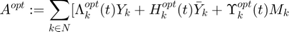
Subject to:
![$$ \sum_{k\in N}[\Lambda_k(t)Y_k+H_k(t)\bar{Y}_k+\Upsilon_k(t)M_k]\geq 0 $$](Opt_OptimalFlow_eq09500839071622004471.png)
Optimization variables in these equations are:
![$$ z_{l}(t):=[z_{l0}(t),z_{l1}(t),z_{l2}(t)]^T $$](Opt_OptimalFlow_eq09867432753565406939.png)
![$$ x(t)=[\lambda^{min}(t)^T, \lambda^{max}(t)^T,
\bar{\lambda}^{min}(t)^T,\bar{\lambda}^{max}(t)^T,\mu^{min}(t)^T,
\mu^{max}(t)^T], l \in G$ and $ t \in T $$](Opt_OptimalFlow_eq01073789375450458547.png)
In these equations,  and
and  are the upper and lower bound for marginal cost of active power for the generators,
  and
and  are the upper and lower marginal cost of reactive power of generators, and
  and
and  are the marginal variables for upper and lower bound of voltages.
clc;
clear all;
close all;
Because of lack of data in 14 bus IEEE test case, I applied the model for 6 bus IEEE test case which is achieved from one of the references. In this test case, we have generator and 6 lines as well as 6 loads. For the first step,  can be calculated from the impedance of branches as follows:
z12=.025+i*.3182;
z24=.2677+i*.1765;
z23=.2839+i*.1931;
z36=.2074+i*.144;
z35=.0611+i*0.0597;

y12=1/z12;
y24=1/z24;
y23=1/z23;
y36=1/z36;
y35=1/z35;
No_bus=6;
Ybus=[y12,-y12,0,0,0,0;
    -y12,y12+y23+y24,-y23,-y24,0,0;
    0,-y23,y23+y35+y36,0,-y35,-y36;
    0,-y24,0,y24,0,0;
    0,0,-y35,0,y35,0;
    0,0,-y36,0,0,y36];
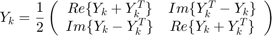
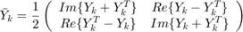
As can be seen in the formulation, we have two  and
and  are calculated as following equations:

for i=1:1:No_bus
    e_matrix=zeros(No_bus,1);
    e_matrix(i,1)=1;
    Mk_matrix(:,:,i)=[e_matrix*transpose(e_matrix), zeros(No_bus,No_bus); zeros(No_bus,No_bus),e_matrix*transpose(e_matrix)];
    Yk=e_matrix*transpose(e_matrix)*Ybus;
    Yk_matrix(:,:,i)=.5*[real(Yk+transpose(Yk)),imag(transpose(Yk)-Yk);imag(Yk-transpose(Yk)),real(Yk+transpose(Yk))];
    Ykvar_matrix(:,:,i)=-.5*[imag(Yk+transpose(Yk)),real(Yk-transpose(Yk));real(transpose(Yk)-Yk),imag(Yk+transpose(Yk))];
end
The load profile for the active and reactive power for 24 hours has been shown in the following figures:
Pd=[0.0031;.0071;.0088;.0082;.0055;.0057];
Qd=[.0023;.0062;.003;.0061;.0029;.006];

load_index=[.5;.42;.42;.4;.42;.48;.6;.62;.52;.48;.47;.46;.43;.4;.47;.5;.58;.85;.93;.9;.88;.8;.63;.53];

t1=1:24;
figure;
hold on
plot(t1,Pd(1)*load_index);
plot(t1,Qd(1)*load_index,'-r');
legend('Active Power','Reactive Power');
title('Power Consumption in Bus#1')
xlabel('Time(h)')
ylabel('Power Consumption (pu)')
grid on;
hold off

The generators on each bus have the maximum and minimum levels for the active and reactive power generation as  and
and  for the active power and
  and
and  for reactive power. Also,
  ,
,  , and
, and  are the generator operational cost coefficients.
Pmax=[.08;0;0;0;0;0];
Pmin=[0;0;0;0;0;0];
Qmax=[.08;0;0;0;0;0];
Qmin=[-.08;0;0;0;0;0];

cl_0=0;
cl_1=14;
cl_2=2;
The upper and lower bound voltage have been noted as  and
and  which are 1.05 and 0.95 pu.
Vmax=1.05;
Vmin=.95;

T=24;

t1=1;
t2=T;

cvx_begin
cvx_solver sedumi
variables lambdaf_min(No_bus,T)
variables lambdaf_max(No_bus,T)
variables lambdavar_min(No_bus,T)
variables lambdavar_max(No_bus,T)
variables muu_min(No_bus,T)
variables muu_max(No_bus,T)
variables lambda(No_bus,T)
variables lambdavar(No_bus,T)
variables muu(No_bus,T)
variables zl_1(T)
variables zl_2(T)
variables h(T)

maximize sum(h)
subject to
for t=t1:t2
    h(t)==sum(lambdaf_min(:,t).*Pmin-lambdaf_max(:,t).*Pmax+lambda(:,t).*Pd*load_index(t)...
        +lambdavar_min(:,t).*Qmin-lambdavar_max(:,t).*Qmax+lambdavar(:,t).*Qd*load_index(t)...
        +muu_min(:,t).*(Vmin.^2)-muu_max(:,t).*(Vmax.^2))+cl_0-zl_2(t);
    lambda(1,t)*Yk_matrix(:,:,1)+lambdavar(1,t)*Ykvar_matrix(:,:,1)+muu(1,t)*Mk_matrix(:,:,1)...
        +lambda(2,t)*Yk_matrix(:,:,2)+lambdavar(2,t)*Ykvar_matrix(:,:,2)+muu(2,t)*Mk_matrix(:,:,2)...
        +lambda(3,t)*Yk_matrix(:,:,3)+lambdavar(3,t)*Ykvar_matrix(:,:,3)+muu(3,t)*Mk_matrix(:,:,3)...
        +lambda(4,t)*Yk_matrix(:,:,4)+lambdavar(4,t)*Ykvar_matrix(:,:,4)+muu(4,t)*Mk_matrix(:,:,4)...
        +lambda(5,t)*Yk_matrix(:,:,5)+lambdavar(5,t)*Ykvar_matrix(:,:,5)+muu(5,t)*Mk_matrix(:,:,5)...
        +lambda(6,t)*Yk_matrix(:,:,6)+lambdavar(6,t)*Ykvar_matrix(:,:,6)+muu(6,t)*Mk_matrix(:,:,6)==semidefinite(2*No_bus);
    zl_2(t)-zl_1(t)*zl_1(t)>=0;
The constraints for this state has been updated for  as follow:

lambda(1,t)==-lambdaf_min(1,t)+lambdaf_max(1,t)+cl_1+2*sqrt(cl_2).*zl_1(t);

    for i=2:No_bus
        lambda(i,t)==-lambdaf_min(i,t)+lambdaf_max(i,t);
    end

lambdavar(:,t)==-lambdavar_min(:,t)+lambdavar_max(:,t);

muu(:,t)==-muu_min(:,t)+muu_max(:,t);
All variables should be positive as follows:


    lambdaf_min(:,t)>=0;
    lambdaf_max(:,t)>=0;


    lambdavar_min(:,t)>=0;
    lambdavar_max(:,t)>=0;


    muu_min(:,t)>=0;
    muu_max(:,t)>=0;


    zl_1(t)>=0;
    zl_2(t)>=0;
end
cvx_end
cvx_optval
Calling SeDuMi 1.34: 2880 variables, 936 equality constraints
   For improved efficiency, SeDuMi is solving the dual problem.
------------------------------------------------------------
SeDuMi 1.34 (beta) by AdvOL, 2005-2008 and Jos F. Sturm, 1998-2003.
Alg = 2: xz-corrector, Adaptive Step-Differentiation, theta = 0.250, beta = 0.500
eqs m = 936, order n = 1273, dim = 4465, blocks = 49
nnz(A) = 4488 + 0, nnz(ADA) = 15192, nnz(L) = 8064
 it :     b*y       gap    delta  rate   t/tP*  t/tD*   feas cg cg  prec
  0 :            1.12E-01 0.000
  1 :  -8.35E+01 3.75E-02 0.000 0.3359 0.9000 0.9000   2.53  1  1  1.3E+01
  2 :  -1.55E+01 1.34E-02 0.000 0.3573 0.9000 0.9000   1.95  1  1  2.9E+00
  3 :  -3.71E+00 3.43E-03 0.000 0.2565 0.9000 0.9000   1.97  1  1  4.8E-01
  4 :  -1.00E+00 1.04E-03 0.000 0.3032 0.9000 0.9000   1.23  1  1  1.3E-01
  5 :  -2.65E-01 3.04E-04 0.000 0.2923 0.9000 0.9000   1.02  1  1  4.0E-02
  6 :  -1.54E-01 1.31E-04 0.000 0.4298 0.9000 0.4553   0.76  1  1  2.1E-02
  7 :   4.40E-02 5.75E-05 0.000 0.4396 0.9000 0.9380   0.25  1  1  1.9E-02
  8 :   2.11E-01 3.56E-05 0.000 0.6195 0.5241 0.9000  -0.58  1  1  1.8E-02
  9 :   6.86E-01 2.34E-05 0.000 0.6579 0.9000 0.9000  -0.45  1  1  1.5E-02
 10 :   1.70E+00 1.20E-05 0.000 0.5105 0.9000 0.9000  -0.21  1  1  1.1E-02
 11 :   2.71E+00 7.65E-06 0.000 0.6393 0.9000 0.9000  -0.24  1  1  9.1E-03
 12 :   4.07E+00 5.05E-06 0.000 0.6598 0.9000 0.9000   0.18  1  1  6.5E-03
 13 :   6.37E+00 1.46E-06 0.000 0.2889 0.9000 0.9000   0.64  1  1  2.0E-03
 14 :   7.21E+00 2.86E-07 0.000 0.1962 0.9000 0.9000   0.92  1  1  4.1E-04
 15 :   7.37E+00 6.07E-08 0.000 0.2122 0.9000 0.9000   0.99  1  1  8.7E-05
 16 :   7.40E+00 1.20E-08 0.000 0.1983 0.9000 0.9000   1.00  1  1  1.7E-05
 17 :   7.41E+00 4.28E-09 0.000 0.3560 0.9000 0.9000   1.00  1 54  6.2E-06
 18 :   7.41E+00 1.53E-09 0.000 0.3571 0.9000 0.9000   1.00  1 73  2.2E-06
 19 :   7.41E+00 5.50E-10 0.000 0.3595 0.9000 0.9000   1.00  1 79  8.0E-07
 20 :   7.41E+00 1.10E-10 0.000 0.1995 0.9000 0.9000   1.00  1 99  1.6E-07
 21 :   7.41E+00 2.59E-12 0.000 0.0236 0.9900 0.9900   1.00  1 99  3.8E-09

iter seconds digits       c*x               b*y
 21      2.2   Inf  7.4118293390e+00  7.4118293433e+00
|Ax-b| =   3.2e-08, [Ay-c]_+ =   0.0E+00, |x|=  2.4e+01, |y|=  5.6e+02

Detailed timing (sec)
   Pre          IPM          Post
6.030E-01    2.251E+00    1.800E-02
Max-norms: ||b||=1.102500e+00, ||c|| = 9.899495e+00,
Cholesky |add|=240, |skip| = 0, ||L.L|| = 77.4317.
------------------------------------------------------------
Status: Solved
Optimal value (cvx_optval): +7.41183


cvx_optval =

    7.4118
for t=t1:t2
There exists an optimal solution for this problem  and a matrix which can get us voltage and power generation of generators as follows:
has a zero eigen value of multiplicity of two for  .
.
Aopt(:,:,t)=lambda(1,t)*Yk_matrix(:,:,1)+lambdavar(1,t)*Ykvar_matrix(:,:,1)+muu(1,t)*Mk_matrix(:,:,1)...
    +lambda(2,t)*Yk_matrix(:,:,2)+lambdavar(2,t)*Ykvar_matrix(:,:,2)+muu(2,t)*Mk_matrix(:,:,2)...
    +lambda(3,t)*Yk_matrix(:,:,3)+lambdavar(3,t)*Ykvar_matrix(:,:,3)+muu(3,t)*Mk_matrix(:,:,3)...
    +lambda(4,t)*Yk_matrix(:,:,4)+lambdavar(4,t)*Ykvar_matrix(:,:,4)+muu(4,t)*Mk_matrix(:,:,4)...
    +lambda(5,t)*Yk_matrix(:,:,5)+lambdavar(5,t)*Ykvar_matrix(:,:,5)+muu(5,t)*Mk_matrix(:,:,5)...
    +lambda(6,t)*Yk_matrix(:,:,6)+lambdavar(6,t)*Ykvar_matrix(:,:,6)+muu(6,t)*Mk_matrix(:,:,6);
In order to get the values for votlage buses, we need to use the singular vetor decomposition as follow. In this command, we can get two vectors  and a diagonal matrix as
  . From the vectors corresponding to the zero eigen values, we can get the voltage of each bus. These voltages should be adjusted to 1.05 value same as follow. Also, in this analysis, we calculated the loss power and operating cost due to this generation.
[U,S,V]=svd(Aopt(:,:,t));
V_slack=U(1:6,12)+1i*U(7:12,12);
Voltage(:,t)=1.05*V_slack/abs(V_slack(1,1));
Pg(t)=(lambda(1,t)-cl_1)/(2*cl_2);
Ploss(t)=Pg(t)-sum(Pd*load_index(t));
Cost(t)=cl_2*Pg(t)*Pg(t)+cl_1*Pg(t)+cl_0;
end
Numerical Result
This section illustrates methods for solving the OPF problem which are described in Section Problem Formulation, on a small-scale example shown in Figure 1. A detailed specification of the considered network parameters are given in [1], for the base voltage rating 10 kV and the base power rating 100 MVA. We tried to consider battery for this case, but there was an error about the feasibility of solutions (it means that the optimal value was infinity). Because of this reason, we removed the battery for the analysis, and tried to complete the model for the 6 bus IEEE test case as [1].
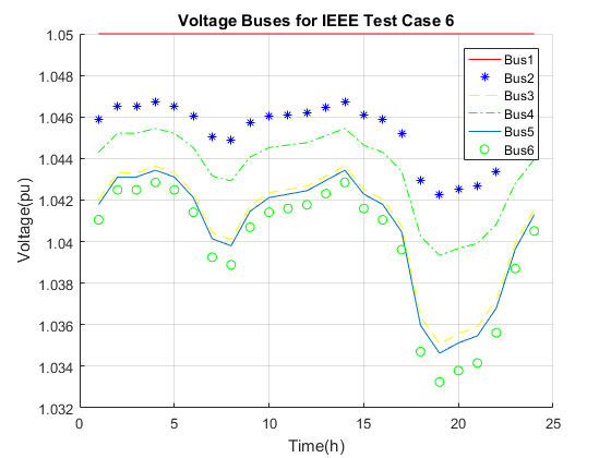
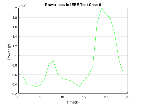
Consider the OPF problem where the objective is to minimize cost function of generators injected at slack bus 1. The figure for votlage can be proven by the Table II in [1]. For more analysis, we put some figures about the operation cost and loss power for this test case. As can be seen, with the increment of demand, the loss power and generation power have been increased.
t=1:1:T;
Abs_Voltage=abs(Voltage);

figure;
hold on
plot(t,Abs_Voltage(1,:),'-r');
plot(t,Abs_Voltage(2,:),'*b');
plot(t,Abs_Voltage(3,:),'--y');
plot(t,Abs_Voltage(4,:),'-.g');
plot(t,Abs_Voltage(5,:));
plot(t,Abs_Voltage(6,:),'go');
legend('Bus1','Bus2','Bus3','Bus4','Bus5','Bus6');
title('Voltage Buses for IEEE Test Case 6');
xlabel('Time(h)');
ylabel('Voltage(pu)');
grid on;
hold off

figure;
hold on
plot(t,Pg,'r');
title('Power Generation in Bus#1')
xlabel('Time(h)')
ylabel('Power (pu)')
grid on;
hold off

figure;
hold on
plot(t,Ploss,'g');
title('Power loss in IEEE Test Case 6')
xlabel('Time(h)')
ylabel('Power (pu)')
grid on;
hold off

figure;
hold on
plot(t,Cost,'y');
title('Operating Cost in IEEE Test Case 6')
xlabel('Time(h)')
ylabel('Cost($/pu)')
grid on;
hold off


Conclusion
The optimal power flow problem has been a fundamental problem in power system operation and analysis for well over half a century. This simulation gave a short review of recent advances in convexification methods for solving the OPF problem, which were developed in a last few years. These methods proved to be very promising, since they can often provide a globally optimal solution of the highly nonconvex OPF problem.
Reference
[1] Novoselnik, Branimir. "Convex Relaxations of Optimal Power Flow."
[2] Lavaei, Javad, and Steven H. Low. "Convexification of optimal power flow problem." Communication, Control, and Computing (Allerton), 2010 48th Annual Allerton Conference on. IEEE, 2010.
[3] Lavaei, Javad, and Steven H. Low. "Zero duality gap in optimal power flow problem." IEEE Transactions on Power Systems 27.1 (2012): 92-107.
[4] Gayme, Dennice, and Ufuk Topcu. "Optimal power flow with large-scale storage integration." IEEE Transactions on Power Systems 28.2 (2013): 709-717.