ECE 602 - Project - A convex framework for image segmentation with moment constraints
by Shitij Vasist and Jobanmeet Kaur
based on the paper by Maria Klodt, Daniel Cremers, "A convex framework for image segmentation with moment constraints", IEEE International Conference, 2011.
Contents
Introduction
Convex relaxation techniques have become a popular approach to image segmentation as they allow to compute solutions independent of initialization to a variety of image segmentation problems. The aim of this project is to interactively partition the main object from a digital picture, separating it from the background. The method used to track the object is based on the intensity histograms. Histogram-based methods are much more efficient when compared to other image segmentation methods as they ordinarily require just one pass through the pixels. The histogram is computed using all the pixels in the image using the intensity as the measure.
Problem Formulation
In this project, we focus on a class of functionals of the form:
where  denotes a hyper surface in
  , i.e. a set of closed boundaries in the case of 2D image segmentation. The functions
  and
and  are application dependent. In a statistical framework for image segmentation, for example,

may denote the log likelihood ratio for observing the color  at a point
  given that is part of the background or the object, respectively.
Shape Optimization via Convex Relaxation
Functionals of the form (1) can be globally optimized in a spatially continuous setting by means of convex relaxation and thresholding. To this end, one reverts to an implicit representation of the hyper surface using an indicator function  on the space of binary functions of bounded variation, where
  and
and  denote the interior and exterior of . The functional (1) defined on the space of surfaces is therefore equivalent to the functional
where the second term in (2) is the weighted total variation. Here  denotes the distributional derivative which for differentiable functions boils down to
  . By relaxing the binary constraint and allowing the function
  to take on values in the interval between 0 and 1, the optimization problem becomes that of minimizing the convex functional (2) over the convex set
  . Global minimizers
  of this relaxed problem can therefore efficiently be computed, for example by a simple gradient descent procedure.
The tresholding theorem assures that thresholding the solution of the relaxed problem preserves global optimality for the original binary labeling problem. We can therefore compute global minimizers for functional (2) in a spatially continuous setting as follows: Compute a global minimizer of (2) on the convex set and threshold the minimizer at any value  .
.
Proposed Solution
Shape optimization and image segmentation can now be done by minimizing convex energies under respective convex constraints.
Let  be a specific convex set containing knowledge about respective moments of the desired shape—given by an intersection of the above convex sets. Then we can compute segmentations by solving the convex optimization problem

with  given in (2). In this project we solved the Euler-Lagrange equations using the lagged diffusivity approach.
Discretization of the Euler-Lagrange equation leads to a sparse nonlinear system of equations, which can be solved via gradient descent. However, gradient descent converges very slowly. Thus, we used a fixed point iteration scheme that transforms the nonlinear system into a sequence of linear systems. These can be efficiently solved with iterative solvers, such as Gauss-Seidel, successive over-relaxation (SOR), or even multi-grid methods. The only source of nonlinearity is the diffusivity  . For constant g, it yields a linear system of equations, which we solve with the SOR method. An update step for at pixel
  and time step
  yields
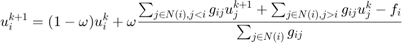
where  is the diffusivity between pixel and
  , and
, and  is the 4-connected neighborhood around i. The vector
  contains the constant part of the equation that does not depend on , i.e. the fidelity term
 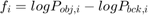 . The method converges for overrelaxation parameters
  . We obtained the fastest convergence rate for
  .
.
In the case of segmentation without moment constraints, there is only the constraint that  , where we project such that
 ![$u \in [0,1]$](optiproj_eq13599045985247151713.png) . This constraint can be enforced by clipping the values of at every point after each iteration:
. This constraint can be enforced by clipping the values of at every point after each iteration:
Code and Figures
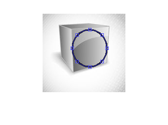
%The user marks an ellipse at approximate size and location of the object
% with mouse click
close all;
im=imread('grayscale.jpg');
im = rgb2gray(im);
figure, imshow(im);

h = imellipse;
logicalmask = h.createMask();
Iterative updates to improve u(x)
for it = 1:80
    % Acquiring the object and background and computing probability
    % densities
    objectmask = uint8(logicalmask);
    backgroundmask = uint8(imcomplement(logicalmask));

    obj = im.*objectmask;
    bkg = im.*backgroundmask;
    pobj = imhist(obj(logicalmask))/numel(obj(logicalmask));
    pbkg = imhist(bkg(imcomplement(logicalmask)))/numel(bkg(imcomplement(logicalmask)));

    %f(x) denotes the log likelihood ratio for observing the color I(x) at
    %a point x
    applyprob = @(x) probDensity(x,pobj,pbkg);

    f = arrayfun(applyprob,im);
    u = double(logicalmask);
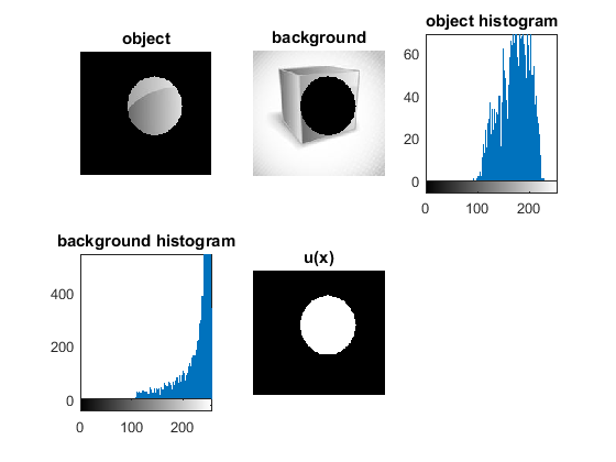
First Iteration Plots
    if(it==1)
    figure
    subplot(2,3,1)
    imshow(obj)
    title('object')
    subplot(2,3,2)
    imshow(bkg)
    title('background')
    subplot(2,3,3)
    imhist(obj(logicalmask))
    title('object histogram')
    subplot(2,3,4)
    imhist(bkg(imcomplement(logicalmask)))
    title('background histogram')
    subplot(2,3,5)
    imshow(u)
    title('u(x)')
    end
    [dux,duy] = gradient(u);
    du = [dux duy];
    absdu(it) = norm(du(:),2);

    %updating u(x) by calculating diffusivities with neighbours and
    %plugging in the values mentioned in the formula above.

    [row,col] = size(u);

    for i = 1:row
        for j = 1:col
            if(i==1)
                g1=0;
            else
                g=gradient(u(i-1:i,j));
                g1 = 1/norm(g(:),2);
            end
            if(i==row)
                g2=0;
            else
                g=gradient(u(i:i+1,j));
                g2 = 1/norm(g(:),2);
            end
            if(j==1)
                g3=0;
            else
                g=gradient(u(i,j-1:j));
                g3 = 1/norm(g(:),2);
            end
            if(j==col)
                g4=0;
            else
                g=gradient(u(i,j:j+1));
                g4 = 1/norm(g(:),2);
            end
            sum = 0;
            sumg = 0;
            if(g1~=0 && ~isinf(g1))
                sum = sum + g1*unew(i-1,j);
                sumg = sumg + g1;
            end
            if(g2~=0 && ~isinf(g2))
                sum = sum + g2*u(i+1,j);
                sumg = sumg + g2;
            end
            if(g3~=0 && ~isinf(g3))
                sum = sum + g3*unew(i,j-1);
                sumg = sumg + g3;
            end
            if(g4~=0 && ~isinf(g4))
                sum = sum + g4*u(i,j+1);
                sumg = sumg + g4;
            end
            w=1.85;
            if(sum>0)
                unew(i,j) = (1-w)*u(i,j) + w*(sum - f(i,j))/sumg;
            else
                unew(i,j) = u(i,j);
            end
        end
    end

    %clipping u(x) to lie within our boundaries
    applyprob = @(x) clipu(x);
    unew = arrayfun(applyprob,unew);
    logicalmask = logical(unew);
end
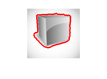
Segmentation Result
figure
bw2 = imfill(uint8(unew), 'holes');
bw2 = edge(uint8(unew),'canny');
bw2 = imdilate(bw2,strel('disk',2));
[B,L] = bwboundaries(bw2,'noholes');
imshow(im)
hold on
for k = 1:length(B)
   boundary = B{k};
   plot(boundary(:,2), boundary(:,1), 'r', 'LineWidth', 3)
end
Results and Analysis
For all experiments we use  and
and 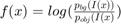 with input image
  . We compute the likelihoods
  and
and  using gray-scale histograms from inside and outside regions defined by the user input. The segmentation without constraint results are consistent with the results in the paper.
The appearance of Infs was frequent and hence the algorithm was tailored to tackle issues related to it.
Linked Files
Function probDensity
function [ y ] = probDensity( x , pobj, pbkg)
% Function to compute the log likelihood ratio for observing color I(x) at a point x

if x~=0 && pobj(x)~=0 && pbkg(x)/(pobj(x))~=0
    y = (log(pbkg(x)/(pobj(x))));
else
    y=0;
end
end
Function clipu
function [ y ] = clipu( x )
% Clipper function that clips u(x) outside of our boundaries

if(x<0)
    y = 0;
elseif x > 1
    y=1;
else
    y=round(x);
end
end