ECE 602 FINAL PROJECT - Convex Optimization Strategies for Coordinating Large-Scale Robot Formations
Pranav Ganti (20663913), Leonid Koppel (20433722)
Contents
Introduction
Multi-robot teams are becoming increasingly viable as a solution in a variety of different fields, due to advances in wireless communications and embedded computing. Potential applications include surveillance, search and rescue, or military operations. Dr. Jason Derenick and Dr. John Spletzer, in their paper "Convex Optimization Strategies for Coordinating Large-Scale Robot Formations" [1], investigate the use of convex optimization strategies to coordinate these multi-agent teams. This problem can be formulated as a a Second-Order Cone Program (SOCP), and either the maximum distance or total distance travelled by these robots between formations can be minimized. In this project, we look to use CVX to solve these SOCPs, and implement the extensions proposed by the authors, such as additional workspace constraints and path-planning in a polygonal environment.
Problem Formulation
Consider  robots in a plane with initial pose
  . We want the robots to move to a final pose
  which is similar to
  - that is, having the same shape up to translation, rotation, and scale. This similarity is denoted by
  . We constrain scale to be positive, disallowing reflection.
The two related problems are as follows: given an initial pose  , choose
  to either
minimize  , the maximum distance travelled; or
minimize  , the total distance travelled
where  and
and  represent the coordinates of each point in the initial and final pose. The desired shape is represented by
  .
.
Note that we do not consider the assignment problem, the problem of choosing which robot corresponds to which  in the target shape. We only find the optimal translation, orientation, and scale of the shape given a fixed correspondence. This problem is convex, while the assignment problem is not.
Additionally, we reproduce two extensions demonstrated in the original paper: adding polygonal workplace constraints, and motion planning through an environment defined as a series of polygons. These problems are formulated in later sections.
Proposed solution
Derenick and Spletzer start with the constraints on the final pose, given the desired shape. The constraints are, for  :
:
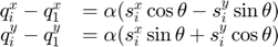
These constraints simply express an affine transformation of the target shape. We can thus express them as affine functions.
Here there appears to be an omission in Derenick and Spletzer's paper. They specify  , and state, "without loss of generality, we can define the formation orientation and scale, repectively, as"

However, the above expression for  is only valid if we also define
  . That is, the target shape must be expressed such that the first two points lie on the horizontal axis. Otherwise, it is impossible for , which obviously expresses a relationship between and , to be independent of . We obtained incorrect results until we added this requirement, which is demonstrated in the Analysis section.
With the requirement in place, the affine form of the constraints is found to be
for  . Note that there are
  constraints, leaving four free variables: the 2D translation, rotation, and scale of the target shape.
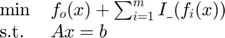
The constraints can be expressed in the matrix form  . Then the problems are

Using the epigraph form, the problems can be restated as second-order cone programs:
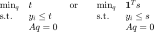
where 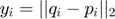 ,
,  ,
,  .
.
In this report, we demonstrate only the second problem, minimizing total distance. This matches the demonstrations in the original paper.
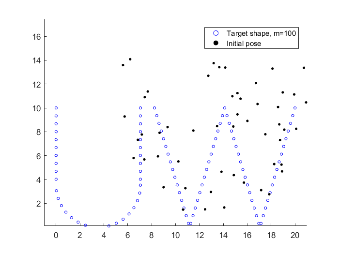
Data synthesis
For our reproduction, we used a shape repesenting the letters "UW". We generate points for any by interpolating along a series of curves representing the letters, as implemented in UW_points.m.
m = 100;
S = UW_points(m);
We produce the initial pose by arbitrarily transforming the shape, and adding random noise to each point. We do this because, as noted above, the assignment problem is not addressed; this way, we start with a somewhat sensible assignment where each robot's initial point  is correlated to its target point. This appears to be what Derenick and Spletzer did in their paper, as choosing completely random does not produce such pleasing results.
p_theta = -pi/2 + 0.2;
p_scale = 1;
R = [cos(p_theta) sin(p_theta); -sin(p_theta) cos(p_theta)];
p_trans = [5 10];
P = p_scale * S*R + p_trans; % Transform
P = P + 6*rand(m,2); % Add uniform random noise
An example is presented below:
figure(1); clf;
plot_shape;
Solution
To implement the constraints in matrix form , we let  be the "flattened" vector form of , where odd elements represent
  -values and even elements represent
  -values. Then
 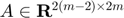 . The matrix
  is generated in constraint_matrix.m
A = constraint_matrix(S);
Here we formulate the problem to minimize total distance:
cvx_begin quiet
variable q(2*m) % vector form of q: odd elements x, even elements y
Q = reshape(q, 2, m)'; % matrix form, each row has (x, y) point
y = norms(Q-P, 2, 2);  % y_i = || q_i - p_i ||_2
variable t(m)   % auxiliary variable for epigraph form

minimize ones(1,m) * t
subject to
    y <= t
    A*q == 0
cvx_end
Results
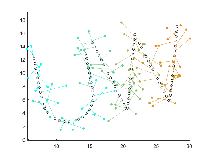
The figure below shows the initial pose (filled circles) and the final pose (empty black circles) which forms the target shape while minimizing total distance travelled, represented by line segments.
figure(2); clf;
plot_robots(P, Q);
Integrating Workspace Constraints
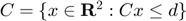
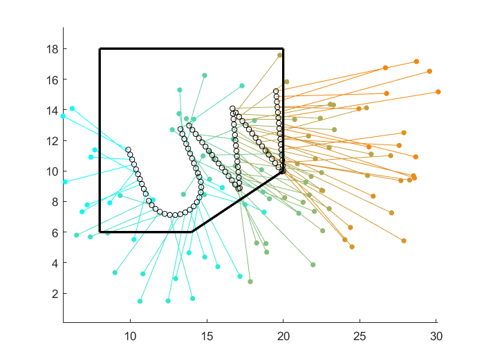
An additional constraint that can be implemented is that of a "workspace constraint". A convex shape, such as a polyhedron, can be integrated as a constraint for the final configuration to lie within. The workspace C can be expressed as:
For the purpose of demonstration, let us specify an arbitrary 5-sided polyhedron which lies within the original operating environment.
The 5 equations which specify the polyhedra are as follows:


This would be placed into the following matrix inequality:
 , with:
A_c = [0 -1;
       0  1;
       1  0;
      -1 0;
       2/3 -1];

b_c = [-6, 18, 20, -8, 10/3]';
Once again, we formulate the problem to minimize total distance:
cvx_begin quiet
variable q(2*m) % vector form of q: odd elements x, even elements y
Q = reshape(q, 2, m)'; % matrix form, each row has (x, y) point
y = norms(Q-P, 2, 2);  % y_i = || q_i - p_i ||_2
variable t(m)   % auxiliary variable for epigraph form

minimize ones(1,m) * t
subject to
    y <= t
    A*q == 0

    % The following inequalities constrain the workspace to the polyhedron
    % defined above.
    for i = 1:m
        A_c*Q(i, :)' <= b_c;
    end
cvx_end
The figure below shows the final pose minimizing total distance travelled, constrained to the arbitrary workspace (black lines). The initial pose is the same as before.
figure(3); clf;
plot_robots(P, Q);
draw_polyhedron;
We can see here now that the optimal robot locations are constrained within the polyhedron.
Notes on Complexity
One of Derenick and Spletzer's contributions to this paper was the formulation of this problem in a manner that can be solved efficiently, even as the number of robots increases past 1000.
To do this, however, they first look to reformulate the problem as a inverse log-barrier problem. We can recall from Boyd that the log-barrier method is an interior-point method, which works to solve equality constraints using Newton's method. A barrier method can be formulated as:
where  represents the indicator function for the inequality constraint. For the log-barrier method, however, the indicator function is replaced with the log function, which acts as a sufficient approximation. As per Boyd, this implicitly defines the inequality constraints, with only the equality constraints explicitly stated.
As seen above, the minimum total distance problem had been reformulated in epigraph form. This has been illustrated by Derenick and Spletzer as follows:
where and  have been previously defined. Derenick and Spletzer define the variable
  as the "inverse log-barrier scaler for the kth iteration". This has been defined as:
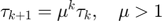
We believe that this is a typo in the paper;  should be defined as either
  , or
, or  .
.
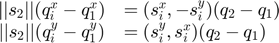
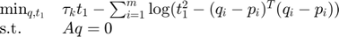
This formulation alone, however, is not sufficient for scalability. In order to maintain O(m) complexity with an increasing number of robots, Derenick and Spletzer reformulate the Karush-Kuhn-Tucker system as a monobanded system; the full derivation for this is discussed within the paper. The final set of constraints are then defined as:
\\
\quad &||s_{2}||_{2}(q_{l}^y - d_{j}^y) = [s_{l}^y, s_{l}^x](d_{j+1} -
d_{j})\\
\quad &t_{i + 1} = t_{i}, \quad i = 1, \ldots, m-1\\
\quad &d_{2i + 1} = d_{2i-1}, \quad i = 1, \ldots, m-3\\
\quad &d_{2(i+1)} = d_{2i}, \quad i = 1, \ldots, m-3\\
\quad &d_{i} = q_{i},\: i \in {1, 2}
\end{array}
$$](main_eq03182269656734911033.png)
for  and
and 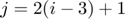 .
.
This formulation of the problem is not solvable using CVX. The objective function actually violates the Disciplined Convex Programming (DCP) ruleset, as the log function consists of two convex terms being summed together; CVX deems this an illegal operation. It would be possible to write a custom solver, but since this section merely describes an optimized method of solving the same problem, we feel that it is outside the scope of the ECE 602 Final project.
Motion planning in polygonal environments
Derenick and Spletzer extend the above problem by considering a robot formation moving through a polygonal environment. We assume we already have a map of the environment decomposed into triangles, such that any two consecutive triangles form a convex region, and that a path through  triangles has been found by some high-level planner. We seek to find a path for each robot which minimizes the total distance travelled while maintaining formation and not colliding with the environment.
The constraints for each triangle are expressed as three halfspace inequalities of the form  .
.
We generate a randomized environment with 16 triangles and the corresponding constraints in the functions below.
k = 16; % number of triangles
triangles = generate_env(k);
[C,d] = triangle_constraints(triangles);
There is a slight hitch: in this problem, the optimal path tends toward  , thus a minimum scale constraint is desired. Unfortunately, while maximum scale constraints are convex, a minimum scale constraint of the form

is not in convex (recall 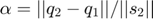 , thus its sublevel sets but not superlevel sets are convex).
Spletzer's earlier work [2] includes an approximation scheme to allow a minimum scale constraint, but also notes that a scale constraint is convex if orientation is fixed.
For this demonstration we use the latter approach, and set a fixed orientation, which appears to be what Derenick and Spletzer used for their demonstration. Following their example, we use a circular formation of robots, generating the points in circle_points.m. We place the initial pose inside the first triangle.
m = 12; % number of robots
S = circle_points(m);
P = 3*S - [5.5 1];
We formulate the problem as
where 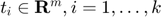 . This is expressed in CVX below.
min_scale = 2;
PrevQ = P;

cvx_begin quiet
variable q(2*m, k-1) % vector form of q, for each triangle 1..k
variable scale nonnegative
Q = reshape(q, 2, m, k-1); % matrix form, with 3rd dimension for each triangle
Q = permute(Q, [2 1 3]);
variable t(m, k-1)   % auxiliary variable for epigraph form

minimize sum(t(:))
subject to
    for i = 1:k-1
        % Minimize total distance
        norms(Q(:,:,i) - PrevQ, 2, 2) <= t(:, i);
        % Constrain shape with fixed orientation
        for j = 2:m
            Q(j,:,i) - Q(1,:,i) == scale * S(j,:)
        end
        % Constraint to inside triangle
        for j = 1:m
             C(:,:,i+1) * Q(j,:,i)' <= d(:,:,i+1)
        end
        % Constraint minimum scale
        scale >= min_scale

        PrevQ = Q(:,:,i);
    end
cvx_end
Results
The below figure presents the polygonal environment (black dashed lines) and the optimal sequential path which minimizes total distance travelled while avoiding collisions. Orientation and minimum scale of the robot formation are constrained.
figure(4); clf;
plot_triangles(triangles);
plot_robot_path(P, Q);
Analysis
We were able to recreate the results obtained by the authors. However, we identified an unstated assumption in the paper. This section will discuss that finding in detail, and then discuss the applications and limitations of the work in general.
Limitation on
The main objective of this paper was to formulate swarm robotic motion as a convex optimization problem, where the swarm of robots maintained a "shape", the "geometric information that remains when location, scale, and rotational effects are removed". Derenick and Spletzer's definition for the formation orientation, , is incorrect without the additional choice  .
.
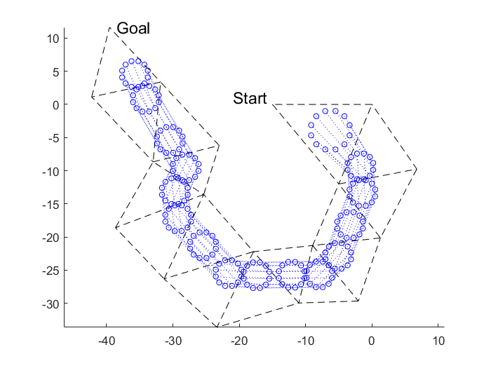
Shown below is the simplest example illustrating this shortcoming. Let us construct a triangle, with vertices at (0,0), (0, 1), and (1,0). The initial location of the robots are directly at the vertices of the shape. In theory, the robots should already be at their optimal location, and no motion should be required.
% Define triangle shape
sx = [0, 0, 1];
sy = [0, 1, 0];
S = [sx; sy]';

% Define number of points
m = 3;

% Define initial position to be exactly the location of the shape
px = sx;
py = sy;
P = [px; py]';

% Define constraint matrix
A = constraint_matrix(S);
Here we formulate the problem to minimize total distance:
cvx_begin quiet
variable q(2*m) % vector form of q: odd elements x, even elements y
Q = reshape(q, 2, m)'; % matrix form, each row has (x, y) point
y = norms(Q-P, 2, 2);  % y_i = || q_i - p_i ||_2
variable t(m)   % auxiliary variable for epigraph form

minimize ones(1,m) * t
subject to
    y <= t
    A*q == 0
cvx_end

figure(5);
clf; hold on;
plot_triangle_example(Q, P, S);
Clearly, this result is incorrect. The expected result is that the final pose (blue stars) and initial pose (red circles) are identical. For comparison, if the vertices in the shape are defined as:
sx = [0, 1, 0];
sy = [0, 0, 1];
S = [sx; sy]';
That is, the 2nd point is (1,0) instead of (0,1), we see that the solution is correctly determined.
figure(6);
openfig('expected_triangle_example.fig');
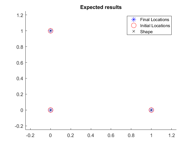
This demonstrates that the requirement is important. Note this choice can still be made without loss of generality; it just requires that the representation of the target shape ,$s$, be correctly rotated when the problem is formulated.
Limitations in our reproduction
We only demonstrated the solution for the "total distance" problem, though the paper also formulates the "minimax" distance problem. However, only the former problem was demonstrated in the figures in the paper. Since the solutions are very similar, our implementation could easily be changed to solve the minimax problem.
We did not reproduce the optimization discussed in the "Notes on Complexity" section. However, we found that our solution for minimum total distance, as implemented in CVX, took approximately 0.15 seconds of CPU time for  . This matches the authors' result for their optimized algorithm. This suggests that a decade's worth of CPU advances can make up for a less efficient implementation. (Of course, an opmimized algorithm would still be faster, especially for greater ).
Applications and limitations
The optimization methods demonstrated can be useful for controlling a swarm of robots, but have several shortcomings. These shortcomings mostly stem from considering only convex optimization problems.
First, Derenick and Spletzer's method does not address the assignment problem. For example, if the initial pose is a uniformly random distribution of robots, we obtain a result similar to one below:
figure(7);
openfig('assignment_problem.fig');
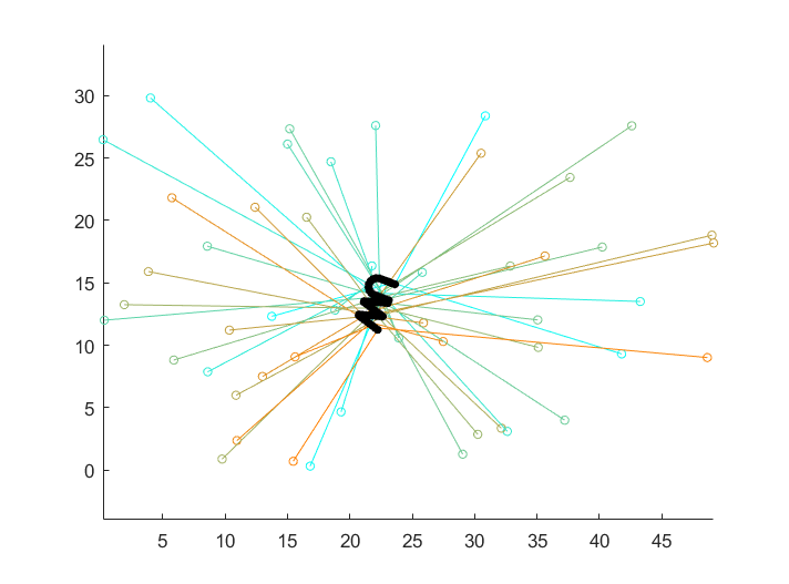
That is, when the assignmentof the robots is completely random, the distance-mininimizing pose tends toward a point in the centre of the initial pose. In a real-world situation, this result is unlikely to be useful, and a better assignment of robots is desired. A suboptimal, approximate assignment may suffice; alternatively, the methods in this paper may be useful as part of a solution for the (nonconvex) assignment problem.
Another limitation, which is noted by the authors, is that the robots' kinematic constraints are not considered. Nonholonomic kinematics, in particular, present a non-convex problem. However, the authors claim, "although the results will no longer be optimal for such robots, they should still be quite good in practice."
The path planning solution also does not consider collisions between the robots. Thus, in practice it can only be used as an input to some lower-level motion planner.
In the path-planning case, the convexity requirement is a considerable drawback: the minimum-scale constraint is convex only if orientation is fixed. In a real-world situation, it is desirable to have a minimum-scale constraint (since robots physically must maintain some distance from each other) and often not desirable to have a fixed orientation. In this case, the approximations proposed in the authors' other work [2] may be useful.
One higher-level limitation of this work is that it assumes a central planner which is aware of all of the robots' positions. In reality, control of the robot swarm may be decentralized.
Some of these limitations are addressed in the authors' later works. For example, [3] addresses collision avoidance between the robots.
Conclusion
We successfully reproduced the results obtained by Derenick and Spletzer for the minimimum total distance problem, and identified an unstated assumption in their derivation. We also reproduced the two extensions demonstrated in the paper: the addition of workspace constraints, and path planning in a polygonal environment. We found the solution to be useful for high-level planning, but too limited to stand alone without additional algorithms for assignment and collision avoidance.
References
- [1] J. Derenick and J. Spletzer, "Convex Optimization Strategies for Coordinating Large-Scale Robot Formations", IEEE Transactions on Robotics, vol. 23, no. 6, pp. 1252-1259, 2007.
- [2] J. Spletzer and R.Fierro, “Optimal positioning strategies for shape changes in robot teams,” in Proc. IEEE Int. Conf. Robot. Automat., 2005, pp. 742– 747.
- [3] J. Derenick, J. Spletzer and V. Kumar, “A Semidefinite Programming Framework for Multi–robot Systems Operating in Dynamic Environments”, Proceedings of the 49th IEEE Conference on Decision and Control (CDC 2010), Atlanta, Georgia, Dec, 2010.
Source code
main.m is the source file used to generate this report.
The following functions are used for data synthesis:
- UW_points.m: generates "UW" shape
- circle_points.m: generates circle shape
- generate_env.m: generates triangular environment
The following functions are used to formulate the optimization problems:
- constraint_matrix.m: formulates matrix for Aq = 0
- triangle_constraints.m: formulates matrices for Cq <= d
The following functions are used for plotting results: