A Convex Optimization Approach to Smooth Trajectories for Motion Planning with Car-Like Robots
Contents
Problem Formulation
Given collision-free waypoints in a maze, our goal is to drive a robot along this trajectory. However, though collision-free is achieved, some parts of the trajectory may be impractical and(or) inefficient for the real robot to move along. Thus, we need to smooth the trajectory, in this demonstration, using convex optimization.
Proposed Solution
- minimization problem: imagine there is an artificial tensile force between points, the aim is to minimize the sum of these forces, subject to friction constraints, turning radius constraints, initial orientation of the vehicle.
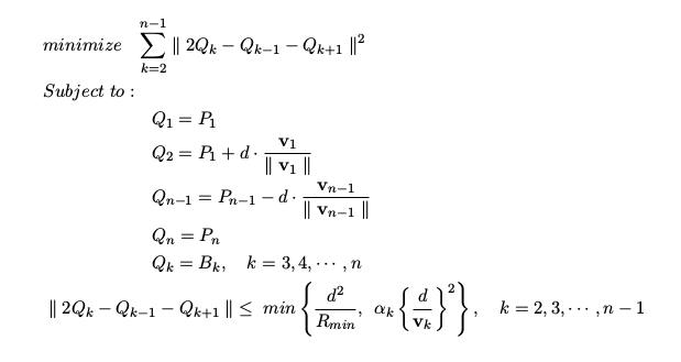
- minimization variable: in the implementation of this algorithm, the optimization variables are those forces represented by the l2-norm of adjacent points.
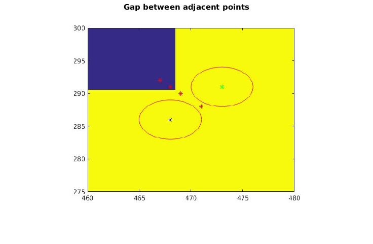
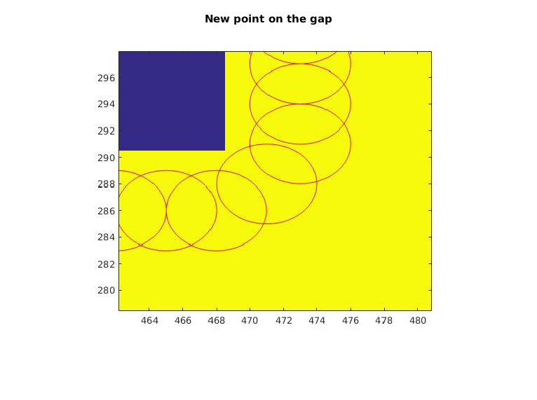
- algorithmic workflow: first, find the collision-free circles of original waypoints. Second, due to fact that the circles found have a great proportion of intersection, this step will sort out some necessary waypoints and their corresponding circles. Third, Check if there is a gap (no intersection) between any two adjacent points. If is, then give a new point to intersect both of its adjacent two points. Fourth, using convex optimization method to smooth the trajectory.
Image Initialization
clc;clear;close all;
I = imread('maze.jpg');
I2 = imbinarize(I(:,:,1), 0.8); % Convert to 0-1 image
% I3 = image_to_binary_map(I2);
I4 = flipud(I2); % To make Y-axis correspond to startpos and endpos
I5 = padarray(flipud(I2),[1,1],0);
Calculate Collision-free Radius of Each Point
load('P.mat'); % load original waypoints
P = flipud(P);
r=[];
for i = 1 : 1 : length(P)
    [r_temp, p_trouble, P(i,:)]= findRadius(P(i,:), I5); % find collision-free circles
    r = [r r_temp];% radius of cicles
end
Sort Out Necessary Points
r_shrkRate = 0.40; % shrink radius of circles by this rate
r_pos = find(r >= (1/2) * max(r));
r(r_pos)= r_shrkRate * max(r);
[sortedPoint, sortedRadius] = sortEffectivePoint(P, r); % sort out necessary points
[P, r] = intervalCheck(sortedPoint, sortedRadius, I5);% check if there is interval
--- 16% points are sorted out!
Initialization of Optimizaiton
d = 0;
n = length(P);
for i = 2 : 1 : n
    d = d + norm(P(i,:) - P(i-1,:), 2);
end
d = d * 1./(n-1); % average distance between two points

R_min = 0.5; % Minimum turning raidus of the vehicle
alpha_k = 3; % coefficient
v_k = [0.5 0.8]; % x and y velocities of the vehicle
friction_cstr = alpha_k * (d/ norm(v_k, 2)).^2; % friction constraints
radius_cstr = d.^2 ./ R_min; % turning radius constraints
Convex Optimization
cvx_begin
    variables Q(n,2) % waypoints to be obtained from optimization
    Q(1,:) == P(1,:);
    Q(2,:) == P(1,:) + d .* 0.6;
    Q(n,:) == P(n,:);
    Q(n-1,:) == P(n,:) - d .* 0.6;
    sum = 0;

    for k = 2 : 1 : n-1
       norm(Q(k, :) - P(k, :), 2) <= r(k); % restrict points inside the collision-free circles
       N_k(k-1) = norm(2.* Q(k, :) - Q(k-1, :) - Q(k+1, :), 2);
       N_k(k-1) <= min(friction_cstr, radius_cstr);
       sum = sum + pow_pos(N_k(k-1),2); % sum of "forces"
    end
       minimize sum
cvx_end
Calling SDPT3 4.0: 6513 variables, 3010 equality constraints
------------------------------------------------------------

 num. of constraints = 3010
 dim. of sdp    var  = 1002,   num. of sdp  blk  = 501
 dim. of socp   var  = 3006,   num. of socp blk  = 1002
 dim. of linear var  = 2004
*******************************************************************
   SDPT3: Infeasible path-following algorithms
*******************************************************************
 version  predcorr  gam  expon  scale_data
   HKM      1      0.000   1        0
it pstep dstep pinfeas dinfeas  gap      prim-obj      dual-obj    cputime
-------------------------------------------------------------------
 0|0.000|0.000|5.6e+01|8.7e+01|1.6e+08| 7.872158e+04  0.000000e+00| 0:0:00| spchol  1  1
 1|0.140|0.228|4.8e+01|6.7e+01|2.0e+08| 2.473138e+05 -2.766712e+06| 0:0:00| spchol  1  1
 2|0.152|0.631|4.1e+01|2.5e+01|1.6e+08| 1.565051e+06 -5.027564e+06| 0:0:00| spchol  1  1
 3|0.879|1.000|4.9e+00|1.3e-01|3.1e+07| 4.143031e+06 -4.699389e+06| 0:0:00| spchol  1  1
 4|0.916|1.000|4.1e-01|6.2e-02|4.1e+06| 5.432318e+05 -2.117849e+06| 0:0:00| spchol  1  1
 5|0.841|0.875|6.5e-02|3.5e-02|7.7e+05| 2.468226e+05 -3.568037e+05| 0:0:00| spchol  1  1
 6|0.914|0.850|5.6e-03|3.2e-02|1.7e+05| 4.312772e+04 -1.198722e+05| 0:0:00| spchol  1  1
 7|1.000|0.902|6.6e-10|8.4e-03|5.5e+04| 2.061117e+04 -3.375167e+04| 0:0:00| spchol  1  1
 8|0.968|0.991|1.8e-10|1.5e-03|1.6e+04| 5.851150e+03 -9.864357e+03| 0:0:01| spchol  1  1
 9|0.946|0.940|1.4e-10|4.9e-04|4.8e+03| 2.830499e+03 -1.995117e+03| 0:0:01| spchol  1  1
10|0.970|0.995|4.1e-12|1.3e-04|1.2e+03| 1.531419e+03  3.495598e+02| 0:0:01| spchol  1  1
11|0.913|0.960|3.5e-13|4.2e-05|4.0e+02| 1.238319e+03  8.344531e+02| 0:0:01| spchol  1  1
12|0.939|1.000|2.2e-14|1.1e-05|1.2e+02| 1.126902e+03  1.006499e+03| 0:0:01| spchol  1  1
13|0.965|1.000|3.3e-15|3.4e-06|3.5e+01| 1.089702e+03  1.054873e+03| 0:0:01| spchol  1  1
14|0.969|0.996|3.8e-15|1.0e-06|1.1e+01| 1.079545e+03  1.068587e+03| 0:0:01| spchol  1  1
15|0.970|1.000|3.5e-15|3.1e-07|3.4e+00| 1.076284e+03  1.072876e+03| 0:0:01| spchol  1  1
16|0.915|0.931|9.8e-15|1.1e-07|1.2e+00| 1.075300e+03  1.074092e+03| 0:0:01| spchol  1  1
17|1.000|1.000|4.3e-14|2.8e-08|4.6e-01| 1.074962e+03  1.074500e+03| 0:0:01| spchol  1  1
18|0.976|0.963|2.7e-14|9.0e-09|1.0e-01| 1.074800e+03  1.074700e+03| 0:0:01| spchol  1  1
19|1.000|1.000|4.6e-13|1.0e-12|3.8e-02| 1.074773e+03  1.074734e+03| 0:0:01| spchol  1  1
20|0.887|0.970|1.6e-13|1.0e-12|9.8e-03| 1.074760e+03  1.074750e+03| 0:0:01| spchol  1  1
21|1.000|1.000|3.9e-12|1.0e-12|3.5e-03| 1.074757e+03  1.074753e+03| 0:0:01| spchol  1  2
22|1.000|0.976|5.7e-14|1.0e-12|1.1e-03| 1.074755e+03  1.074754e+03| 0:0:01| spchol  2  1
23|0.710|0.763|1.2e-12|1.2e-12|6.2e-04| 1.074755e+03  1.074755e+03| 0:0:01| spchol  2  2
24|1.000|0.721|9.8e-14|1.3e-12|2.7e-04| 1.074755e+03  1.074755e+03| 0:0:01| spchol  2  1
25|1.000|0.641|1.8e-11|1.5e-12|1.3e-04| 1.074755e+03  1.074755e+03| 0:0:01| spchol  2  2
26|1.000|0.623|2.3e-13|2.1e-12|6.6e-05| 1.074755e+03  1.074755e+03| 0:0:01| spchol  2  2
27|1.000|0.613|2.3e-13|1.8e-12|3.4e-05| 1.074755e+03  1.074755e+03| 0:0:01| spchol  2  2
28|1.000|0.607|3.6e-13|1.7e-12|1.8e-05| 1.074755e+03  1.074755e+03| 0:0:01|
  stop: max(relative gap, infeasibilities) < 1.49e-08
-------------------------------------------------------------------
 number of iterations   = 28
 primal objective value =  1.07475489e+03
 dual   objective value =  1.07475487e+03
 gap := trace(XZ)       = 1.79e-05
 relative gap           = 8.34e-09
 actual relative gap    = 8.32e-09
 rel. primal infeas (scaled problem)   = 3.58e-13
 rel. dual     "        "       "      = 1.71e-12
 rel. primal infeas (unscaled problem) = 0.00e+00
 rel. dual     "        "       "      = 0.00e+00
 norm(X), norm(y), norm(Z) = 1.8e+03, 3.2e+02, 3.4e+02
 norm(A), norm(b), norm(C) = 1.1e+02, 1.8e+03, 2.3e+01
 Total CPU time (secs)  = 1.47
 CPU time per iteration = 0.05
 termination code       =  0
 DIMACS: 8.0e-12  0.0e+00  2.0e-11  0.0e+00  8.3e-09  8.3e-09
-------------------------------------------------------------------

------------------------------------------------------------
Status: Solved
Optimal value (cvx_optval): +1074.75
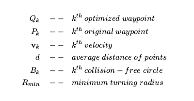
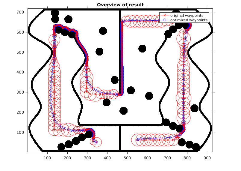
Plot Results
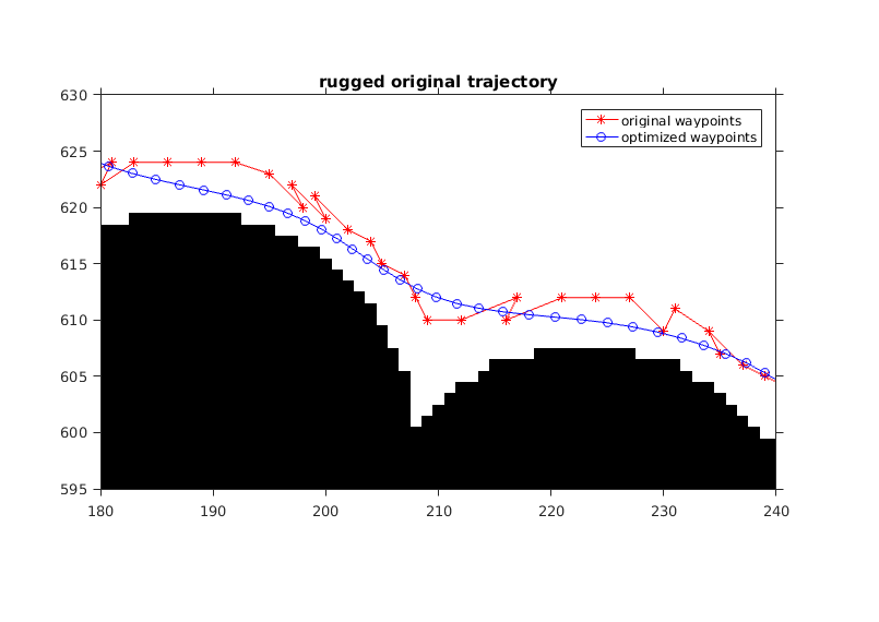
figure(1)
imshow(I5)
title('Overview of result');
hold on
axis on
set(gca,'YDir','normal');
plot(P(:,1), P(:,2),'r-*');
plot(Q(:,1), Q(:,2),'b-o');
for i = 1 : 1 : length(r)
    drawCircle( P(i,:),r(i) );
end
legend('original waypoints','optimized waypoints');

% * *inefficient original trajectory*
figure(2)
imshow(I5)
hold on
axis on
set(gca,'YDir','normal');
title('inefficient original trajectory');
plot(P(:,1), P(:,2),'r-*');
plot(Q(:,1), Q(:,2),'b-o');
legend('original waypoints','optimized waypoints');
axis([100 260 80 180]);

% * *rugged original trajectory*
figure(3)
imshow(I5)
hold on
axis on
set(gca,'YDir','normal');
title('rugged original trajectory');
plot(P(:,1), P(:,2),'r-*');
plot(Q(:,1), Q(:,2),'b-o');
legend('original waypoints','optimized waypoints');
axis([180 240 595 630]);

figure(4)
imshow('intervalCheck.jpg')
title('Gap between adjacent points');
figure(5)
imshow('intervalCheck_2.jpg')
title('New point on the gap');
Warning: Image is too big to fit on screen; displaying at 67%
Warning: Image is too big to fit on screen; displaying at 67%
Warning: Image is too big to fit on screen; displaying at 67%
Analysis and Conclusions
This algorithm succeeds in reproducing the result in the original paper. The origianl paper has two optimization process. One of them is on the trajectory, which we demonstrate in this report, the other process is on the velocity of the vehicle. It, indeed, obtains a smoothed trajectory after the implementation of the algorithm but there are still some points to rethink.
- Ignore robot configuration: The smoothed trajectory is based on the fact that the robot is moving at a constant speed and its heading constrains are ignored
- Check the interval: This algorithm has a new function that is not contained in the thoughts of the original paper. A function inside this algorithm implementation can find out if there is disconnection of any two adjacent points and produce a point compensate for this.
Links and References
[1] Zhijie Zhu, Edward Schmerling, Marco Pavone, "A Convex Optimization Approach to Smooth Trajectories for Motion Planning with Car-Like Robots"
Sources files
- The following custom functions are used
- findRadius.m --- find the raidus of collision-free circle
- drawCircle.m --- draw collision-free circle
- intervalCheck.m --- check if there is gap between any adjacent points
- translatePoint.m --- translate points that are so closed to the obstables
- sortEffectivePoint.m --- sort out some of necessary points