Tensor Completion for Estimating Missing Values in Visual Data

Thibaud Lutellier, 20520400

Contents

Problem Formulation

The aim of this study is to estimate missing values in tensors of visual data.

Problem Solution

To estimate missing values, the authors developed 3 algorithms solving 3 different Convex optimization problems: SiLRTC, FaLRTC and SiLRTC. In this report, we will focus on the SiLRTC algorithm.

Tensor Completion

First, we need to formulate the general Tensor Completion problem as a Convex optimization problem (equation 9 in the paper):

% minimize over X: sum(alpha_i ||X(i)|| ), for i =1 .. n
%
% subject to X_omega = T_omega

Here, X and T are n-mode tensors with identical size in each node. alpha_i are constants >= 0 with the sum of the alpha_i equal to 0.

SiLRTC

The problem above is np-hard to solve when the number of mode (n) is superior to 2. Therefore, a key part of the SiLRTC algorithm is to simplify the problem. To simplify it, they introduce matrices M_1, .. M_n and obtain the equation (15). This is this problem we will attempt to implement.

Data Import

This paper used two kinds of data (synthetic and real world data). I could not find the original images used in the study, therefore, I took screenshots of the original images displayed in the paper and applied similar noise (random white noise) on them (similar to Fig 4,7 and 8). I also did an additional test with removing some writing from the image (I added "ECE 602" with MSPaint on the first image). Compared to the original work, the images will have a different quality, a different size, and the pixel will have slightly different values (as they are screenshots of a PDF file). Most of the results are similar to the results in the paper. The largest difference is with the last image, where parts of the recovered background is gray.

Original Image load

clc;
clear;
close all;

addpath('mylib/');

or_img2= double(imread('testImg2.png'));
or_img3= double(imread('testImg3.png'));
or_img4= double(imread('testImg4.png'));

% Load images with missing values:
T1 = double(imread('testImg1_ece.png')); % Test with non-random noise.

T2 = or_img2;
% Generate 1000 random locations.
numRandom = 1000;
linearIndices = randi(numel(T2)/3, 1, numRandom);
% Set those locations to be "white".
T2(linearIndices) = 255;
T2(linearIndices+numel(T2)/3) = 255;
T2(linearIndices+2*(numel(T2)/3)) = 255;


% 3rd test:
T3 = or_img3;
% Generate 90% of missing random locations.
numRandom3 = int32(0.90*numel(T3)/3);
linearIndices = randi(numel(T3)/3, 1, numRandom3);
% Set those locations to be "white".
T3(linearIndices) = 255;
T3(linearIndices+numel(T3)/3) = 255;
T3(linearIndices+2*(numel(T3)/3)) = 255;

% 4th test:
O = ones(size(or_img4));
T4 = or_img4 -O; %To avoid having values of 255
% Generate 10000 random locations.
numRandom = 10000;
linearIndices = randi(numel(T4)/3, 1, numRandom);
% Set those locations to be "white".
T4(linearIndices) = 255;
T4(linearIndices+numel(T4)/3) = 255;
T4(linearIndices+2*(numel(T4)/3)) = 255;

Parameters for test 1

Omega1 = (T1 < 254); % Barrier for what's considered a missing values. Here, everything that is white is a missing value.
alpha = 1/3; % Coefficients of the objective function, similar to the paper
maxIter = 1000; % maximum iterations
epsilon = 1e-6; % the tolerance of the relative difference of outputs of two neighbor iterations ms(T));
beta = 0.1*ones(1, ndims(T1));   % Relaxation parameter set to 0.1

Solution: SiLRTC for test 1

[X_S1, errList_S1] = SiLRTC(...
    T1,...
    Omega1,...
    alpha, ...
    beta,...
    maxIter,...
    epsilon...
    );

SiLRTC: iterations = 50   difference=0.000093
SiLRTC: iterations = 100   difference=0.000083
SiLRTC: iterations = 150   difference=0.000074
SiLRTC: iterations = 200   difference=0.000067
SiLRTC: iterations = 250   difference=0.000061
SiLRTC: iterations = 300   difference=0.000057
SiLRTC: iterations = 350   difference=0.000052
SiLRTC: iterations = 400   difference=0.000049
SiLRTC: iterations = 450   difference=0.000045
SiLRTC: iterations = 500   difference=0.000043
SiLRTC: iterations = 550   difference=0.000040
SiLRTC: iterations = 600   difference=0.000038
SiLRTC: iterations = 650   difference=0.000035
SiLRTC: iterations = 700   difference=0.000033
SiLRTC: iterations = 750   difference=0.000032
SiLRTC: iterations = 800   difference=0.000030
SiLRTC: iterations = 850   difference=0.000028
SiLRTC: iterations = 900   difference=0.000027
SiLRTC: iterations = 950   difference=0.000025
SiLRTC: iterations = 1000   difference=0.000024
SiLRTC ends: total iterations = 1000   difference=0.000024

Parameters for test 2

Omega2 = (T2 < 254); % Barrier for what's considered a missing values. Here, everything that is white is a missing value.
alpha = 1/3; % Coefficients of the objective function, similar to the paper
maxIter = 500; % maximum iterations
epsilon = 1e-3; % the tolerance of the relative difference of outputs of two neighbor iterations ms(T));
beta = 0.1*ones(1, ndims(T2));   % Relaxation parameter set to 0.1

Solution for test 2

[X_S2, errList_S2] = SiLRTC(...
    T2,...
    Omega2,...
    alpha, ...
    beta,...
    maxIter,...
    epsilon...
    );

SiLRTC ends: total iterations = 1   difference=0.000274

Parameters for test 3

Omega3 = (T3 < 254); % Barrier for what's considered a missing values. Here, everything that is white is a missing value.
alpha = 1/3; % Coefficients of the objective function, similar to the paper
maxIter = 500; % maximum iterations
epsilon = 1e-4; % the tolerance of the relative difference of outputs of two neighbor iterations ms(T));
beta = 0.1*ones(1, ndims(T3));   % Relaxation parameter set to 0.1

Start SiLRTC for test 3

[X_S3, errList_S3] = SiLRTC(...
    T3,...
    Omega3,...
    alpha, ...
    beta,...
    maxIter,...
    epsilon...
    );

SiLRTC: iterations = 50   difference=0.000158
SiLRTC: iterations = 100   difference=0.000154
SiLRTC: iterations = 150   difference=0.000150
SiLRTC: iterations = 200   difference=0.000146
SiLRTC: iterations = 250   difference=0.000142
SiLRTC: iterations = 300   difference=0.000138
SiLRTC: iterations = 350   difference=0.000134
SiLRTC: iterations = 400   difference=0.000131
SiLRTC: iterations = 450   difference=0.000127
SiLRTC: iterations = 500   difference=0.000124
SiLRTC ends: total iterations = 500   difference=0.000124

Parameters for test 4

Omega4 = (T4 < 254); % Barrier for what's considered a missing values. Here, everything that is white is a missing value.
alpha = 1/3; % Coefficients of the objective function, similar to the paper
maxIter = 500; % maximum iterations
epsilon = 1e-5; % the tolerance of the relative difference of outputs of two neighbor iterations ms(T));
beta = 0.1*ones(1, ndims(T4));   % Relaxation parameter set to 0.1

Start SiLRTC for test 4

[X_S4, errList_S4] = SiLRTC(...
    T4,...
    Omega4,...
    alpha, ...
    beta,...
    maxIter,...
    epsilon...
    );

SiLRTC: iterations = 50   difference=0.000236
SiLRTC: iterations = 100   difference=0.000232
SiLRTC: iterations = 150   difference=0.000227
SiLRTC: iterations = 200   difference=0.000221
SiLRTC: iterations = 250   difference=0.000214
SiLRTC: iterations = 300   difference=0.000204
SiLRTC: iterations = 350   difference=0.000191
SiLRTC: iterations = 400   difference=0.000170
SiLRTC: iterations = 450   difference=0.000141
SiLRTC: iterations = 500   difference=0.000109
SiLRTC ends: total iterations = 500   difference=0.000108

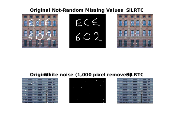
Visualization of Results

figure();
subplot(2,3,1);
imshow(uint8(T1));
title('Original');
subplot(2,3,2);
imshow(double(1-Omega1));
title('Not-Random Missing Values');
subplot(2,3,3);
imshow(uint8(X_S1));
title('SiLRTC');

subplot(2,3,4);
imshow(uint8(T2));
title('Original');
subplot(2,3,5);
imshow(double(1-Omega2));
title('White noise (1,000 pixel removed)');
subplot(2,3,6);
imshow(uint8(X_S2));
title('SiLRTC');

figure();
subplot(2,3,1);
imshow(uint8(T3));
title('Original');
subplot(2,3,2);
imshow(double(1-Omega3));
title('White noise (90% of removed pixels)');
subplot(2,3,3);
imshow(uint8(X_S3));
title('SiLRTC');

subplot(2,3,4);
imshow(uint8(T4));
title('Original');
subplot(2,3,5);
imshow(double(1-Omega4));
title('White noise (10,000 pixel removed)');
subplot(2,3,6);
imshow(uint8(X_S4));
title('SiLRTC');

Analysis: Value of epsilon

Empirically I tested epsilon= 1e-3, 1e-4 and 1e-5 epsilon of 1e-3 is very fast but provide poor results for img1 and img3. It is enough for img2 with just a 1000 missing values. epsilon of 1e-4 provides good results for white noise, even with large values of missing pixels (10,000) but is not so good for the first image. epsilon of 1e-5 provides better results but it takes much more time. In addition, we reach the maximum number of iteration (500) for img 1. Increasing the max number of iteration to 1000 helps, but we still reach the max number of iteration.

Comparison with the results in the paper.

I tested 4 different cases:

First, I took a screenshot of the first image and added text on it with MSPaint. We can see that the algorithm remove the text pretty well, but there are still some artefacts. Note that we reached the maximum number of iteration (1000). Second, we created some white noise by making 1,000 random pixel whites. The algorithm has no issue repairing the image, even with a small epsilon. Third, similarly to the paper, we removed 90% of the pixels of the image. You can see that this algorithm is not perfect for such a corrupted image (we can clearly see some artefacts), despite the image being mostly recovered. Finally, we made some tests on the final image by removing 10,000 pixels. You can see that the image is well recovered, except for the background. The reason is that the background was white. The 2 other more advanced algorithms presented in the paper might be better for large noise.

As I did not have their exact data, I focused especially on the examples for which I could take screenshots directly from the paper. They did not describe precisely how they generated noise in their images, so there might be a difference with my report. Globally, I obtained very similar results. The results of this algorithm for random noise is pretty good.

The paper also reported the execution time of these different algorithms. As I only used one algorithm in this report, I did not replicated this part. The execution time is obviously dependent on the epsilon (acceptable error) and of the max number of iteration when the epsilon can not be reached (see first image). Overall, it took about 15min on my desktop to run everything, most of the time being spent for the first image.

As mentioned earlier, there little difference for the last image of my test. This is likelt due to my screenshots being a bit different compared to the original data. My image has a lot of White background that where from the paper. This white background might not be part of the original image, creating an inconsistency when trying to recover it.

Published with MATLAB® R2015b