Resource Allocation in DataMill: A Performance Evaluation tool

                Introduction to optimization
                         ECE 602
                Course Project - Winter 2017

        Student Name: Waleed Qadir Khan, Anderson Oliveira
                   ID. 20359224 , 20647805

Contents

Problem Formulation

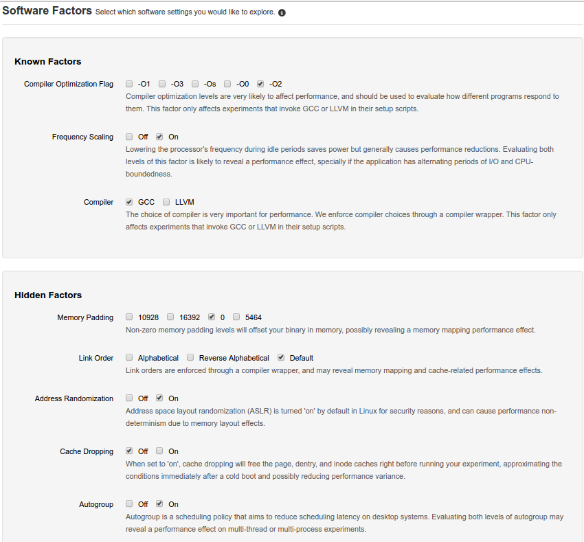
DataMill is a benchmarking and performance evaluation tool developed at the University of Waterloo in collaboration with multiple research groups. DataMill is a distributed infrastructure for computer performance experimentation on real hardware. The infrastructure varies over a selection of hardware and software factors [1]. In this problem, the user must define their experiment for Datamill, which in part consists of which package the code will run on along with constraints specific to the factors under consideration. Through the web interface the user selects all factor levels (e.g. Filesystem type, Compiler optimization level, architecture type, etc.) that should be activated or deactivated during the execution of an experiment. Each worker machine has its own predefined set of factor levels that they are capable of covering and, for this reason, chances are that moderate to complex experiments can not be executed by only one machine. An image of the front-end user interface is given below. After the user has submitted their experiment request, the system then selects the relevant machines capable of executing the experiments on and herein lies the optimization problem. The DataMill infrastructure is composed of a master node, responsible for the distribution of experiment trials and the collection of results, and several worker nodes, which execute the experiment packages provided by the users[1]. Due to the big amount of ongoing experiments and requests, the backend of Datamill has to wisely select the worker machines that cover the factors levels specified by the users. Therefore, the solver's job is to minimize the number of workers necessary to execute the experiments provided the desired coverage. The set of selected workers is represented by a row vector W, and the set of factor levels that will be covered is represented by row vector L

Proposed Solution

The following is the proposed solution outlined in the paper to solve the linear program. The objective function followed by the constraints:

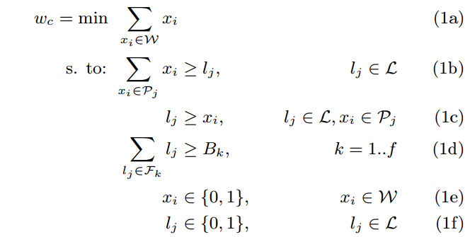
The variables are defined as follows:[1]%

Data Sources

Three pieces of information were required for the program

The data files provided in the submission 'fk_datafile.mat' and 'pm_datafile.mat' are the hardware collected data for points 1 and 2 respectively.

Optimization Solution

The problem is set up as linear, but the one thing to take note of is that the values of the workers and factor levels are either 0 or 1 and choosing a value in the range of 0 to 1 while might solve the optimization problem is not viable since, either a worker is used for the work package or it is omitted and same with the factor level. So the problem is classified as one having integer constraints. Using the default solver provided by CVX (SDPT3) we are solving the relaxed form of the integer constraint problem. Below we have solved the problem both ways using:

Gurobi is a professional optimization solver package that can solve integer constraint problems. We obtained an academic license to the solver and used it as part of our analysis.

Loading the parameters

clear all; close all;


% Load set of factor level. Fk is a matrix which each row represents each
% factor level
Fk = importdata('fk_datafile.mat');

% Load set of machines that provide level m. Pm is a matrix such that each
% row represents the levels a machine support
Pm = importdata('pm_datafile.mat');

% MACHINES_QUANT number of machines
MACHINES_QUANT = 8;

% FACTORS_QUANTITY: Number of factors
FACTORS_QUANTITY = 14;

% LEVEL_QUANTITY: Total number of factor levels
LEVEL_QUANTITY = 44;

Below is an input example of a user-requested minimum coverage for an experiment

frequency_scaling = [1 1]; % Cover frequency saling 'on'  and 'off'
filesystem_type = [0 0 0 0 0 1]; % Cover filesystem BTRFS only
number_of_cores = [0 1 0 0]; % Cover machines with 3 cores
architecture = [0 1]; % Cover x86_64 machines
cpu_clock = [0 0 1 0]; % Select a machine with 2GHz
ram_size = [0 0 0 1 1]; % Select machines with 1 and 2 GB of ram
compiler_type = [1 0]; % Select machines that support GCC
address_randomization = [1 1]; % Cover address randomization ON and OFF
compiler_options = [0 1 0 0]; % Cover complite optimization -O2
memory_padding = [1 0 0 0]; % Cover 0 memory padding
link_order = [0 0 1]; % Cover default link order
cache_dropping = [1 1]; %Cover cache dropping ON and OFF
auto_group = [1 0]; % Cover auto group ON
swap_partition = [1 0]; % Cover swap partition ON

Build vector Bk, the user-requested minimum coverage for factors, for the relaxed constraint problem.

Bk = [sum(frequency_scaling);...
    sum(filesystem_type);...
    sum(number_of_cores);...
    sum(architecture);...
    sum(cpu_clock);...
    sum(ram_size);...
    sum(compiler_type);...
    sum(address_randomization);...
    sum(compiler_options);...
    sum(memory_padding);...
    sum(link_order);...
    sum(cache_dropping);...
    sum(auto_group);...
    sum(swap_partition);...
];

Solving the optimization problem using SDPT3

cvx_solver sdpt3

cvx_begin
    % W is the set of workers
    variable W(MACHINES_QUANT)
    variable L(LEVEL_QUANTITY)

    minimize sum(W)

    subject to

        % ensures picking a factor level means at least one machine with that factor level is added to the solution
        Pm'*W >= L

        % ensures that selecting a machine adds all factor levels it provides to the tally, which is checked
        for j=1:LEVEL_QUANTITY
            for i=1:MACHINES_QUANT
                L(j) >= Pm(i,j)*W(i)
            end
        end

        % Ensures that selecting a machine adds all factor levels it
        % provides to the tally
        Fk*L >= Bk

        % Bounds for relaxed constraints. % Relaxed constraints W E [0,1], L E [0,1]
        0 <= W <= 1
        0 <= L <= 1
cvx_end

% store results
selected_machines_relaxed = W;
selected_levels_relaxed = L;

 
Calling SDPT3 4.0: 514 variables, 52 equality constraints
   For improved efficiency, SDPT3 is solving the dual problem.
------------------------------------------------------------

 num. of constraints = 52
 dim. of linear var  = 514
 12 linear variables from unrestricted variable.
 *** convert ublk to lblk
*******************************************************************
   SDPT3: Infeasible path-following algorithms
*******************************************************************
 version  predcorr  gam  expon  scale_data
    NT      1      0.000   1        0    
it pstep dstep pinfeas dinfeas  gap      prim-obj      dual-obj    cputime
-------------------------------------------------------------------
 0|0.000|0.000|3.1e+02|5.2e+01|2.6e+05| 7.708333e+02  0.000000e+00| 0:0:00| chol  1  1 
 1|0.745|0.373|8.0e+01|3.3e+01|1.6e+05| 3.023604e+03 -2.557773e+01| 0:0:00| chol  1  1 
 2|1.000|0.864|4.8e-05|4.5e+00|3.3e+04| 5.746322e+03 -6.625902e+00| 0:0:00| chol  1  1 
 3|1.000|0.880|2.9e-05|5.7e-01|6.6e+03| 3.996116e+03 -3.447386e+00| 0:0:00| chol  1  1 
 4|0.956|0.805|1.0e-05|1.2e-01|1.5e+03| 1.225189e+03 -3.138607e+00| 0:0:00| chol  1  1 
 5|0.993|0.630|2.9e-07|4.5e-02|2.9e+02| 2.427008e+02 -3.082808e+00| 0:0:01| chol  1  1 
 6|1.000|0.480|2.9e-07|2.4e-02|7.1e+01| 4.653148e+01 -3.014715e+00| 0:0:01| chol  1  1 
 7|0.853|0.904|5.1e-07|2.5e-03|1.2e+01| 7.694261e+00 -2.608172e+00| 0:0:01| chol  1  1 
 8|1.000|0.146|3.4e-06|2.1e-03|9.9e+00| 4.851661e+00 -2.476846e+00| 0:0:01| chol  1  1 
 9|1.000|0.585|4.7e-07|8.9e-04|5.1e+00| 1.877070e+00 -2.093547e+00| 0:0:01| chol  1  1 
10|0.982|0.437|3.9e-08|5.1e-04|2.0e+00|-7.440941e-01 -2.069315e+00| 0:0:01| chol  1  1 
11|0.984|0.959|3.0e-08|2.2e-05|6.3e-02|-1.969019e+00 -2.002162e+00| 0:0:01| chol  1  1 
12|0.989|0.989|1.2e-09|7.9e-07|1.4e-03|-1.999644e+00 -2.000024e+00| 0:0:01| chol  1  1 
13|0.994|0.990|1.1e-10|4.4e-07|1.3e-04|-1.999995e+00 -2.000000e+00| 0:0:01| chol  2  2 
14|1.000|0.989|2.2e-09|3.7e-08|3.1e-06|-1.999999e+00 -2.000000e+00| 0:0:01| chol  2  2 
15|1.000|0.988|9.0e-11|9.1e-10|6.4e-08|-2.000000e+00 -2.000000e+00| 0:0:01|
  stop: max(relative gap, infeasibilities) < 1.49e-08
-------------------------------------------------------------------
 number of iterations   = 15
 primal objective value = -1.99999997e+00
 dual   objective value = -2.00000000e+00
 gap := trace(XZ)       = 6.41e-08
 relative gap           = 1.28e-08
 actual relative gap    = 6.05e-09
 rel. primal infeas (scaled problem)   = 8.99e-11
 rel. dual     "        "       "      = 9.08e-10
 rel. primal infeas (unscaled problem) = 0.00e+00
 rel. dual     "        "       "      = 0.00e+00
 norm(X), norm(y), norm(Z) = 4.7e+02, 5.4e+00, 1.6e+01
 norm(A), norm(b), norm(C) = 3.2e+01, 3.8e+00, 9.8e+00
 Total CPU time (secs)  = 0.58  
 CPU time per iteration = 0.04  
 termination code       =  0
 DIMACS: 1.7e-10  0.0e+00  3.0e-09  0.0e+00  6.0e-09  1.3e-08
-------------------------------------------------------------------
 
------------------------------------------------------------
Status: Solved
Optimal value (cvx_optval): +2
 

Solving the optimization problem using Gurobi

cvx_solver gurobi;

cvx_begin
    % W is the set of workers
    variable W(MACHINES_QUANT) integer
    variable L(LEVEL_QUANTITY) integer

    minimize (sum(W))

    subject to

        % ensures picking a factor level means at least one machine with that factor level is added to the solution
        Pm'*W >= L

        % ensures that selecting a machine adds all factor levels it provides to the tally, which is checked
        for j=1:LEVEL_QUANTITY
            for i=1:MACHINES_QUANT
                L(j) >= Pm(i,j)*W(i)
            end
        end

        % guarantees that all user-provided constraints are met
        Fk*L >= Bk

        % Relaxed constraints W E {0,1}, L E {0,1}
        0 <= W <= 1
        0 <= L <= 1
cvx_end

 
Calling Gurobi 6.00: 566 variables, 514 equality constraints
------------------------------------------------------------
Gurobi optimizer, licensed to CVX for CVX
Optimize a model with 514 rows, 566 columns and 1448 nonzeros
Coefficient statistics:
  Matrix range    [1e+00, 1e+00]
  Objective range [1e+00, 1e+00]
  Bounds range    [0e+00, 0e+00]
  RHS range       [1e+00, 2e+00]
Found heuristic solution: objective 3
Presolve removed 434 rows and 537 columns
Presolve time: 0.00s
Presolved: 80 rows, 29 columns, 480 nonzeros
Variable types: 0 continuous, 29 integer (29 binary)

Root relaxation: objective 2.000000e+00, 34 iterations, 0.00 seconds

    Nodes    |    Current Node    |     Objective Bounds      |     Work
 Expl Unexpl |  Obj  Depth IntInf | Incumbent    BestBd   Gap | It/Node Time

*    0     0               0       2.0000000    2.00000  0.00%     -    0s

Explored 0 nodes (34 simplex iterations) in 0.01 seconds
Thread count was 2 (of 4 available processors)

Optimal solution found (tolerance 1.00e-04)
Best objective 2.000000000000e+00, best bound 2.000000000000e+00, gap 0.0%
------------------------------------------------------------
Status: Solved
Optimal value (cvx_optval): +2
 

Comparison between machines selected by gurobi

(using integer constraints) vs the default cvx solver (with relaxed constraints)

machines_selected_cvx_gurobi = [selected_machines_relaxed W]

machines_selected_cvx_gurobi =

    0.4229    1.0000
    0.3745    1.0000
    0.2628         0
    0.2147         0
    0.1146         0
    0.2913         0
    0.2099         0
    0.1092         0

Comparison between levels selected by gurobi

(using integer constraints) and the default cvx solver (with relaxed constraints)

levels_selected_cvx_gurobi = [selected_levels_relaxed L]

levels_selected_cvx_gurobi =

    1.0000    1.0000
    1.0000    1.0000
    0.8959    1.0000
    0.8790    1.0000
    0.8905    1.0000
    0.5528         0
    0.8860    1.0000
    0.8922    1.0000
    0.9007    1.0000
    0.3745    1.0000
    0.8046    1.0000
    0.4593    1.0000
    0.4694         0
    0.9201    1.0000
    0.0000         0
    0.4229    1.0000
    0.4439         0
    0.8730    1.0000
    0.4229    1.0000
    0.0000         0
    0.0000         0
    0.6875         0
    0.8896    1.0000
    0.9164    1.0000
    0.9141    1.0000
    1.0000    1.0000
    1.0000    1.0000
    0.8721    1.0000
    0.8954    1.0000
    0.8954    1.0000
    0.8922    1.0000
    0.8978    1.0000
    0.7837    1.0000
    0.8228    1.0000
    0.8935    1.0000
    0.8546    1.0000
    0.8784         0
    0.9107    1.0000
    1.0000    1.0000
    1.0000    1.0000
    0.9099    1.0000
    0.9099    1.0000
    0.8876    1.0000
    0.9149    1.0000

Visulizing the data

Worker set choosen by the Gurobi vs Default Solver

Analysis and Conclusions

The authors did not provide graphs or data to compare the results against, however since the DataMill system is available to use, we were able to test out the synthesized data with the actual output. A point to note is that for the purpose of the project, not all machines available to DataMill were added, and as such the test cases developed were such that they were relevant to the selected machine. Our implementation results matched the results generated by the existing system. The interesting part regarding the project was to be able to investigate how the optimization problem is solved when the constrains with respect to W and L are relaxed, how different solvers can be used to solve this problem and what the results provided by the solvers can help us to draw different conclusion about their results. The results show that while both solvers reach the same optimization value, the optimal point of variables W (vector of selected worker machines) and L (vector of factor levels covered) are different. The plots shown above tells us that Gurobi solved the integer constraint problem by choosing two workers for the given set of available workers, while the default solver (used for relaxed constraint problem) choose real values in the range of 0 to 1. If the authors of the paper used the relaxed constraint version to solve the problem, an additional decision strategy (or heuristics) had to be created in order to select the machines amongst the ones selected by the solver. For example, one could decide to select all machines that had its value greater than 0.1. However, if we do not relax the constraints and use gurobi to solve the problem, no additional decision has to be made.

Further Development

During our analysis of the results from our code, we discovered that the factor levels chosen by the solver deviated at times from those prescribed by the user. Further investigating the problem we rooted out the problem to how the problem set up the Bk vector. It combines the user inputs per factor into a scalar and then processes the data. We experience a loss of information in such a structure. We contacted the author of the paper and inquired into the behavior and found out this was a design decision since DataMill does not guarantee 100% level coverage w.r.t to the user input. For the purposes of the project, we decided to improve upon the proposed solution in the paper and extend the functionality so that it does provide 100% line coverage. The following is the proposed updated optimization problem. The entire implementation is provided separately in a file called 'extended_solution.m', but the major changes are shown below

% Build Bk matrix containing the user requested minimum coverage
% Bk = [frequency_scaling zeros(1,42); ...
% zeros(1,2) filesystem_type zeros(1,36); ...
% zeros(1,8) number_of_cores zeros(1,32);...
% zeros(1,12) architecture zeros(1,30);...
% zeros(1,14) cpu_clock zeros(1,26);...
% zeros(1,18) ram_size zeros(1,21);...
% zeros(1,23) compiler_type zeros(1,19);...
% zeros(1,25) address_randomization zeros(1,17);...
% zeros(1,27) compiler_options zeros(1,13);...
% zeros(1,31) memory_padding zeros(1,9);...
% zeros(1,35) link_order zeros(1,6);...
% zeros(1,38) cache_dropping zeros(1,4);...
% zeros(1,40) auto_group zeros(1,2);...
% zeros(1,42) swap_partition];

% cvx_solver gurobi;
%
% cvx_begin
%
%     variable W(MACHINES_QUANT) integer
%     variable L(LEVEL_QUANTITY) integer
%
%     minimize (ones(1,MACHINES_QUANT)*W)
%
%     subject to
%
%
%         Pm'*W >= L
%
%
%         for j=1:LEVEL_QUANTITY
%             for i=1:MACHINES_QUANT
%                 L(j) >= Pm(i,j)*W(i)
%             end
%         end
%
%         for f=1:FACTORS_QUANTITY
%             L'.*Fk(f, :) >= Bk(f, :);
%         end
%
%         0 <= W <= 1
%         0 <= L <= 1
% cvx_end
%

Results

The results of the updated solver corresponded to the same minimization value as the one described before, with the added benefit of achieving 100% level coverage. By using a matrix for the Bk we avoid loss of information to the system and hence can generate more precise constraints that produce the desired results.

Linked files

Following are all the necessary files associated with the project:

References

Published with MATLAB® R2016a