Optimal Downlink Beamforming Using Semidefinite Optimization
Authors: Ararat Shaverdian and Mai Hassan
In this report, we recreate and comment on the results of the paper "Optimal Downlink Beamforming Using Semidefinite Optimization" by Mats Bengtsson and Björn Ottersten [1].
Contents
- 1 Introduction
- 2 Problem formulation
- 3 Data sources
- 4 Solution
- 4.1 Scheme 1: The joint optimal design
- 4.2 Scheme 2: The decentralized heuristic design
- 4.3 Scheme 3: The heuristic generalized eigenvector design
- 4.4 Scheme 4: The traditional beamforming design
- 5 Visualization of results
- 6 Analysis and conclusions
- 7 References
1 Introduction
Beamforming is the use of antenna arrays to point the main lobe of the transmitted signal from a base station in the direction of a specific receiver (or user). This allows for the suppression of the interfering signals (from other users) to each specific user. In this project, we present a number of beamforming array (or vector) design problems in the form of optimization problems. Specifically, we compare two alternative beamforming optimization solutions (proposed in [1]) to two established solutions in the literature. The first proposed solution is a joint optimal design where each base station jointly optimizes its users' beamforming vectors. The second solution is a decentralized heuristic (sub-optimal) approach where the base station determines each user's beamformers independently of the other users'.
The proposed solutions ensure the minimization of the total transmitted power while maintaining a pre-determined quality of service for each user.
2 Problem formulation
The first solution is a centralized optimization problem that minimizes the total transmitted power such that the received signal-to-interference-and-noise-ratio (SINR) at each user  is above a certain threshold, i.e.,
  . The corresponding non-convex optimization problem is as follows:
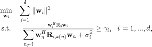
where  and
and  are the beamforming vector and channel covariance matrix (from BS
  ) of user , respectively, and
  denotes the Hermitian of . For simplicity, we use
  instead of
  . The above-mentioned problem provides a lower-bound (in terms of minimum transmit power) on all the other beamforming schemes since it is fully centralized and, hence, the best that can be done in terms of array design for a given set of SINR constraints.
The second proposed solution is a decentralized problem. This is more suitable for real-time networks since it eliminates the intra/inter base station overhead communication required in the centralized problem and, hence, is considered a heuristic approach. Clearly, this is a sub-optimal solution (compared to the centralized one). The proposed solution is formulated as a non-convex optimization problem in the following:
where  . The above-mentioned problem ensures that the received signal-to-noise ratio of each user is above a pre-tuned threshold
  and interference signal caused by each user is below the pre-tuned threshold
  .
.
Note that to be able to solve both of the problems above using the available optimization tools, e.g., CVX, we first need to convexify them. We present the convexified versions of both problems in Section 4 as we present our source code for simulations.
3 Data sources
In the simulation setup, we assume that there are three users served by a single base station (in a given cell) where one of the users is located at  relative array broadside and the other two at directions
  , where the separation angle
  varies from
  to
to  . The transmitting antenna array is linear and has
  elements spaced half a wavelength apart. Each user is surrounded by a large number of local scatterers corresponding to a spread angle of
  , seen from the base station. In all cases, the beamformers are scaled, if possible, such that
  for all users. In the cases where no such scaling is possible for a given
  , the scaling is chosen such that all users receive the same and as high an SINR as possible. The SINR threshold is set to
  dB for each user and, for simplicity, we assume that
  dB for the decentralized problem.
clc;
clear all; %remove all variables, globals, functions and MEX links

%Input Parameters
d = 3; % number of users
m = 8; % number antenna elements
theta = zeros(3,1); % line of sight angle
sigma_theta = 2*pi/180; % spread angle
R = zeros(m,m,d); % covariance matrix
gamma = 10; % sinr threshold 10 dB
sigma_i_sqaured = 1; %The noise variance

delta = 5:25;% The delta of the position of the direction

%Output Parameters:
P1 =zeros(1,length(delta)); % Total transmitted power for scheme(strategy)1
P2 =zeros(1,length(delta)); % Total transmitted power for scheme(strategy)2
P3 =zeros(1,length(delta)); % Total transmitted power for scheme(strategy)3
P4 =zeros(1,length(delta)); % Total transmitted power for scheme(strategy)4

SINR1 = 10*ones(d,length(delta));% SINR per user for scheme(strategy)1
SINR2 = 10*ones(d,length(delta));% SINR per user for scheme(strategy)2
SINR3 = 10*ones(d,length(delta));% SINR per user for scheme(strategy)3
SINR4 = 10*ones(d,length(delta));% SINR per user for scheme(strategy)4

%Maximum SINR thershold used for Scheme 4 in dB, its prederminted by a linear
%search code for delta < 13, otherwise its set to 10 dB
gamma4 = [ -0.4130 0.5220 1.5183 2.5760 3.7245 5.0241 6.5628 8.4440 10 10 10 10 10 10 10 10 10 10 10 10 10];
The  -th element of the channel covariance matrix for a given
  is given as
![$$[\mathbf{R}(\theta, \sigma_{\theta})]_{kl}= e^{j \pi(k-l)sin\theta}e^{-\frac{(\pi(k-l)\sigma_{\theta}cos\theta)^{2}}{2}}.$](Main_eq63408.png)
Below is the code used to generate the covariance matrix  .
.
for ind=1:length(delta) % looping over all values of delta
    theta(1) = 10; theta(2) = 10 + delta(ind); theta(3) = 10 - delta(ind); % theta 1-3 for a given delta

    for theta_indx = 1:d %Generating the channel covariance matrix
        for k = 1:m
            for l = 1:m
                R(k,l,theta_indx) = ...
                    exp( pi*(k-l)*sind(theta(theta_indx))*1i ) ...
                    * exp( -( (pi*(k-l)*sigma_theta*cosd(theta(theta_indx)) )^2 )/2 );
            end
        end
    end
4 Solution
We compare the performance of the following four schemes in terms of the maximum supportable SINR for each user and total transmitted power for a given .
- The joint optimal (centralized) design
- The decentralized heuristic design
- The heuristic generalized eigenvector beamformer
- Traditional Beamforming
4.1 Scheme 1: The joint optimal design
This scheme corresponds to the centralized design introduced in Section 2. To convexify the centralized problem, the authors in [1] introduce the matrices  , use the rule
 ![$\mathbf{w}^H_i \mathbf{R} \mathbf{w}_i = \textrm{Tr}[\mathbf{R}\mathbf{w}_i \mathbf{w}^H_i]$](Main_eq23884.png) and relax the rank one constraint on
and relax the rank one constraint on  . Incorporating these properties into the original (non-convex) centralized problem results in the following "approximated" version which we refer to as Scheme 1.
![$$
\begin{array} {cl}
\displaystyle \min_{\mathbf{W}_i} & ~\displaystyle \sum_{i=1}^{d} \textrm{Tr}[\mathbf{W}_i] \\
\textrm{s.t.} & ~ \textrm{Tr}[\mathbf{R}_i\mathbf{W}_i] -\gamma_i\displaystyle \sum_{n\neq i} \textrm{Tr} [\mathbf{R}_{i,\kappa(n)}\mathbf{W}_n] = \gamma_i\sigma^2_i, \\
&~\mathbf{W}_i^H = \mathbf{W}_i,\\
&~\mathbf{W}_i \succeq 0, ~~ i=1,...,d.\\
\end{array}
$$](Main_eq08552.png)
Notes:
- Since we relax (a.k.a., eliminate) the rank one constraint on , the problem above provides a lower-bound (and, hence, an approximation) to the original centralized problem. This lower-bound is equal to the objective of the original problem, only if all the resulting 's (from Scheme 1) are of rank one.
- The SINR inequalities in the original problem are changed to equality constraints in Scheme 1 to maintain equal SINR at each user; otherwise, if required, one can change the equalities back to inequalities.
The following shows the simulation code for Scheme 1.
    cvx_begin sdp quiet
    variable W(m,m,d) complex hermitian;
    expression total_power;
    total_power =   trace(W(:,:,1)) ...
        + trace(W(:,:,2)) ...
        + trace(W(:,:,3));

    minimize total_power
    subject to
    for i = 1:d
        trace( R(:,:,i)*W(:,:,i) ) - gamma*( ...
            trace( R(:,:,i)*W(:,:,1) ) + ...
            trace( R(:,:,i)*W(:,:,2) ) + ...
            trace( R(:,:,i)*W(:,:,3) ) - ...
            trace( R(:,:,i)*W(:,:,i) ) ) == gamma * sigma_i_sqaured;
        W(:,:,i) == hermitian_semidefinite(m);
    end
    cvx_end

    %output total_power
    P1(ind) = total_power;
    cvx_clear;   % Clear previous CVX variables
4.2 Scheme 2: The decentralized heuristic design
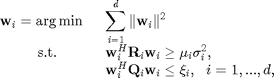
By applying the same mathematical tricks as in the centralized problem, the decentralized problem in Section 2 can be recast as the following convex optimization problem which we refer to as Scheme 2.
![$$
\begin{array} {cl}
\mathbf{W}_i = \arg \min ~ & \textrm{Tr} [\mathbf{W}_i] \\
~ \textrm{s.t.} & \textrm{Tr} [\mathbf{W}_i \mathbf{R}_i] \geq \mu_i \sigma^2_i,\\
& \textrm{Tr}[\mathbf{W}_i\mathbf{Q}_i] \leq \xi_i, \\
& \mathbf{W}_i^H = \mathbf{W}_i, \\
& \mathbf{W}_i \succeq 0, ~~ i=1,...,d. \\
& \end{array}
$$](Main_eq67711.png)
Note that the system performance under Scheme 2 depends on the values of  and
and  . Since these values are not specified in [1], we use a linear search to approximate them (Recall that we keep
  dB).
dB).
The following shows the simulation code for Scheme 2.
    if (delta(ind)>=8.5)
        %Fine-tune the parameter eta
        if delta(ind) == 11
            eta = 10^3/3;
        elseif delta(ind) == 11.5
            eta = 10^3/2.5;
        elseif 9 <= delta(ind) && delta(ind) < 10
            eta = 10^3/4;
        elseif delta(ind) == 10 || delta(ind) == 10.5 || delta(ind) == 12
            eta = 10^3;
        else
            eta = 10^3/5;
        end

        mu = 10 * eta / sigma_i_sqaured; % set mu

        V = zeros(m,m,d); % instantiate matrix V to save W's in
        total_power = 0; % instantiate power variable

        % Solve the decentralized problem, i.e., the eq. below eq. (12) in the
        % paper
        for i = 1:d
            cvx_begin sdp quiet
            variable W(m,m,d) complex hermitian;
            minimize trace( W(:,:,i) )
            subject to
            trace( W(:,:,i)*R(:,:,i) ) >= mu * sigma_i_sqaured;
            trace( W(:,:,i)*( R(:,:,1)+R(:,:,2)+R(:,:,3)-R(:,:,i) ) ) <= eta;
            W(:,:,i) == hermitian_semidefinite(m);
            cvx_end
            V(:,:,i) = W(:,:,i);
            cvx_clear
        end

        % scale the weight matrices so that every user receives an SINR of
        % exactly 10 dB
        cvx_begin sdp quiet
        variable scaler(d,1);
        subject to
        for i = 1:d
            scaler(i)*trace( R(:,:,i)*V(:,:,i) ) - gamma*( ...
                scaler(1)*trace( R(:,:,i)*V(:,:,1) ) + ...
                scaler(2)*trace( R(:,:,i)*V(:,:,2) ) + ...
                scaler(3)*trace( R(:,:,i)*V(:,:,3) ) - ...
                scaler(i)*trace( R(:,:,i)*V(:,:,i) ) ) == gamma * sigma_i_sqaured;
            scaler >= 0;
        end
        cvx_end

        % update the weights according to their corresponding scalars
        for i = 1:d
            scaler(i)*trace( R(:,:,i)*V(:,:,i) ) / ( ...
                scaler(1)*trace( R(:,:,i)*V(:,:,1) ) + ...
                scaler(2)*trace( R(:,:,i)*V(:,:,2) ) + ...
                scaler(3)*trace( R(:,:,i)*V(:,:,3) ) - ...
                scaler(i)*trace( R(:,:,i)*V(:,:,i) ) + sigma_i_sqaured );
        end

        P2(ind) = scaler(1)*trace(V(:,:,1)) + ...
            scaler(2)*trace(V(:,:,2)) + ...
            scaler(3)*trace(V(:,:,3));
    end
4.3 Scheme 3: The heuristic generalized eigenvector design
In the next two sections, we introduce two conventional beamforming heuristic methods to compare the proposed beamforming schemes 1 and 2 to.
The first conventional heuristic is based on the following selection which we refer to as Scheme 3.
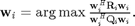
where  and
and ![$\alpha = (0.1/m) \textrm{Tr}[ \sum_{n \neq i }^{d} {\mathbf{R}_{n}}].$](Main_eq64776.png)
The equation above has a very intuitive meaning; the base station selects the beamforming vector (for each user independently) that maximizes the ratio between the received signal and interference caused to other users. The solution to the  equation above (as derived in [2]) is the generalized eigenvector corresponding to the matrix pair
  .
.
The following is the code to simulate Scheme 3. Recall that the 's obtained from the equation above are scaled to ensure that the received SINR at each user is equal and as high as possible. These scaling factors are obtained by solving a system of linear equations as shown in the code. For  , the optimal received SINR thresholds (for a given ) are determined by a linear search code; otherwise, they are set to 10 dB.
    %Choosing the approperiate value of gamma
    if (delta (ind)==5)
        gamma3 =10.^(5.5348/10);
    elseif (delta (ind)== 6)
        gamma3 = 10.^(7.1564/10);
    elseif (delta(ind)==7)
        gamma3= 10.^(8.6542/10);
    else
        gamma3 = gamma;
    end
    for i=1:d
        SINR3(i,ind) = gamma3;
    end

    w = zeros(m,d); % Beamforming vector

    alpha = zeros(d,1); % Arbitrarily variable
    R_i = zeros(m, m, d); % Interference covariance matrix

    % Calculating the interference covariance matrix
    for n=1:d
        for k=1:d
            if (n~=k)
                R_i(:,:,n) = R_i(:,:,n) + R(:,:,k);
            end
        end
    end

    % Calculating of alpha the arbitrarily variable
    for i =1:d
        alpha(i,1) = 0.1*trace(R_i(:,:,i))/m;
    end

    % Calculating the beamforming weight vector based on reference [2]
    for i = 1:d
        Q =  alpha(i,1)*eye(8,8)+R_i(:,:,i);
        [V,D] = eig(R(:,:,i),Q);
        [row,col] = find(D == max(max(D)));
        w(:,i) = V(:,col);
    end

    % Scaling the total transmit power to achieve the required SINR thershold
    % (gamma) by solving a 3x3 linear system of equations
    syms x y z

    % SINR for first user
    eqn1 = x*(w(:,1)'*R(:,:,1)*w(:,1)) - gamma3*( ...
        x*( w(:,1)'*R(:,:,1)*w(:,1)) + ...
        y*( w(:,2)'*R(:,:,1)*w(:,2) ) + ...
        z*( w(:,3)'*R(:,:,1)*w(:,3) ) - ...
        x*( w(:,1)'*R(:,:,1)*w(:,1) ) ) == gamma3 * sigma_i_sqaured;

    % SINR for second user
    eqn2 = y*(w(:,2)'*R(:,:,2)*w(:,2)) - gamma3*( ...
        x*( w(:,1)'*R(:,:,2)*w(:,1)) + ...
        y*( w(:,2)'*R(:,:,2)*w(:,2) ) + ...
        z*( w(:,3)'*R(:,:,2)*w(:,3) ) - ...
        y*( w(:,2)'*R(:,:,2)*w(:,2) ) ) == gamma3 * sigma_i_sqaured;

    % SINR for third user
    eqn3 = z*(w(:,3)'*R(:,:,3)*w(:,3)) - gamma3*( ...
        x*( w(:,1)'*R(:,:,3)*w(:,1)) + ...
        y*( w(:,2)'*R(:,:,3)*w(:,2) ) + ...
        z*( w(:,3)'*R(:,:,3)*w(:,3) ) - ...
        z*( w(:,3)'*R(:,:,3)*w(:,3) ) ) == gamma3 * sigma_i_sqaured;

    [A,B] = equationsToMatrix([eqn1, eqn2, eqn3], [x,y,z]);

    scaler = double( linsolve(A,B) );% the scaling factor per user to maintain the SINR thershold required

    % Obtaining the total transitted power
    P3(ind) = real(scaler(1)*w(:,1)'*w(:,1) + ...
        scaler(2)*w(:,2)'*w(:,2) + ...
        scaler(3)*w(:,3)'*w(:,3));
4.4 Scheme 4: The traditional beamforming design
For the second conventional beamforming, we use the traditional beamforming design which is based on the following equation. We refer to this as Scheme 4.
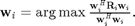
The intuition behind the scheme is to maximize the received-signal-to-transmit-signal ratio. The solution to this equation is the principle eigenvector of [3].
The following shows the simulation code for Scheme 4. Recall that the 's obtained from the equation above are scaled to ensure that the received SINR at each user is equal and as high as possible. The scaling factors are obtained by solving a system of linear equations. For  , the optimal received SINR thresholds (for a given ) are determined by a linear search code; otherwise, they are set to 10 dB.
    w = zeros(m,d);% Beamforming vector

    %Calculating the beamforming weight vector based on the eigenvector of
    %the channel covariance matrix
    for i = 1:d
        [V,D] = eig( R(:,:,i) );
        [row, col] = find( D == max(max(D)) );
        w(:,i) = V(:,col);
    end

    % Scaling the total transmit power to achieve the required SINR thershold
    % (gamma) by solving a 3x3 linear system of equations
    syms x y z

    % SINR for first user
    eqn1 = x*(w(:,1)'*R(:,:,1)*w(:,1)) - 10^(gamma4(ind)/10)*( ...
        x*( w(:,1)'*R(:,:,1)*w(:,1)) + ...
        y*( w(:,2)'*R(:,:,1)*w(:,2) ) + ...
        z*( w(:,3)'*R(:,:,1)*w(:,3) ) - ...
        x*( w(:,1)'*R(:,:,1)*w(:,1) ) ) == 10^(gamma4(ind)/10) * sigma_i_sqaured;

    % SINR for second user
    eqn2 = y*(w(:,2)'*R(:,:,2)*w(:,2)) - 10^(gamma4(ind)/10)*( ...
        x*( w(:,1)'*R(:,:,2)*w(:,1)) + ...
        y*( w(:,2)'*R(:,:,2)*w(:,2) ) + ...
        z*( w(:,3)'*R(:,:,2)*w(:,3) ) - ...
        y*( w(:,2)'*R(:,:,2)*w(:,2) ) ) == 10^(gamma4(ind)/10) * sigma_i_sqaured;

    % SINR for third user
    eqn3 = z*(w(:,3)'*R(:,:,3)*w(:,3)) - 10^(gamma4(ind)/10)*( ...
        x*( w(:,1)'*R(:,:,3)*w(:,1)) + ...
        y*( w(:,2)'*R(:,:,3)*w(:,2) ) + ...
        z*( w(:,3)'*R(:,:,3)*w(:,3) ) - ...
        z*( w(:,3)'*R(:,:,3)*w(:,3) ) ) == 10^(gamma4(ind)/10) * sigma_i_sqaured;

    [A,B] = equationsToMatrix([eqn1, eqn2, eqn3], [x,y,z]);

    scaler = double( linsolve(A,B) );% the scaling factor per user to maintain the SINR thershold required

    % Obtaining the total transitted power
    P4(ind) = real(scaler(1)*w(:,1)'*w(:,1) + ...
        scaler(2)*w(:,2)'*w(:,2) + ...
        scaler(3)*w(:,3)'*w(:,3));

    for i=1:d
        SINR4(i,ind) = 10^(gamma4(ind)/10);
    end
end
5 Visualization of results
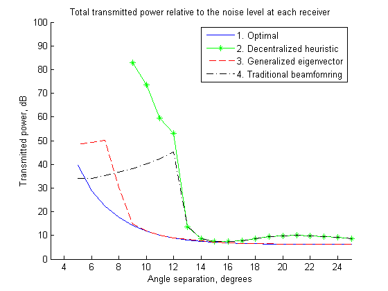
In the first figure, we plot the total transmitted power relative to the noise level at each receiver as a function of the angle separation where the total transmitted power is determined by computing 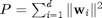 . The following code is used to generate the plot.
hold on;
axis([3 25 0 100]);
plot(delta,10.*log10(P1));
plot(delta,10.*log10(P2),'g *-');
plot(delta,10.*log10(P3),'r --');
plot(delta,10.*log10(P4),'k -.');
title('Total transmitted power relative to the noise level at each receiver')
ylabel('Transmitted power, dB')
xlabel('Angle separation, degrees')
legend('1. Optimal','2. Decentralized heuristic','3. Generalized eigenvector','4. Traditional beamfomring');
hold off;
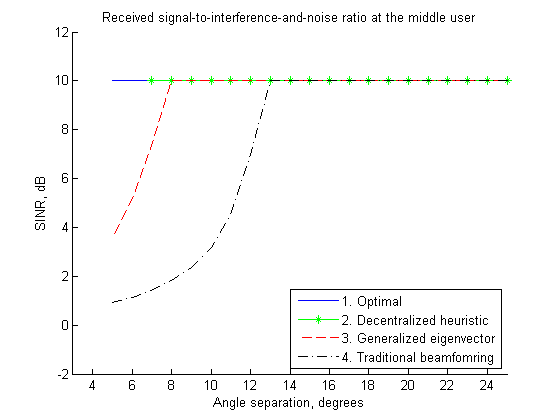
In the second figure, we plot the received SINR at the middle user (i.e., the one with broadside angle of  ) as a function of the angle separation . The following is the code used to generate the figure.
figure
hold on;
axis([3 25 -2 12]);
plot(delta,SINR1(2,:));
plot(7:25,SINR2(2,3:length(delta)),'g *-');
plot(delta,SINR3(2,:),'r --');
plot(delta,SINR4(2,:),'k -.');
title('Received signal-to-interference-and-noise ratio at the middle user')
ylabel('SINR, dB')
xlabel('Angle separation, degrees')
legend('1. Optimal','2. Decentralized heuristic','3. Generalized eigenvector','4. Traditional beamfomring', 'Location','southeast');
hold off;
6 Analysis and conclusions
In conclusion:
- We successfully regenerated all the results in [1].
- In Scheme 1, although the results provide a lower-bound to the original problem (since they correspond to the relaxed version of the original problem), we observe that for medium to high separation angles () the performance of the lower-bound is almost identical to those of schemes 2, 3 and 4 (all of which are sub-optimal). Hence, the lower-bound is tight and a very good approximation to the original (unrelaxed) problem.
- In scheme 2, the total transmitted power graph is not identical to that in [1] for
 , since and require vey precise fine-tuning and their values used in [1] are not specified there. In terms of performance, Scheme 2 outperforms Scheme 3 in terms of maximum supportable SINR for low values of . However, considering the fact that Scheme 3 is much faster to implement in real-time networks (since it only requires the computation of the maximum generalized eigenvector of a pair of matrices), the SINR improvement in Scheme 2 can be seen as a modest advantage over Scheme 3.
 - In terms of performance, Scheme 3 by far appears to be the most efficient solution out of the four schemes because of its practicality (since it is easy to compute) and good performance.
- Scheme 4 exhibits a similar performance to that of Scheme 2 for
 ; for lower values of , Scheme 2 outperforms Scheme 4 in terms of maximum supportable SINR at each user. However, one should note that Scheme 4 is much simpler in terms of implementation costs since it does not require fine-tuning of any parameters and is easy to compute (as opposed to Scheme 2).
 - A major drawback of the paper under study [1] is the lack of enough details on the simulation setup and paramaters used. For example, in the beginning, it was very unclear to us as to how the weight vectors are scaled. Furthermore, the lack of a table to show the optimal values used for and made the simulation task extremely cumbersome. We faced a similar issue when trying to fine-tune the optimal SINR threshold (to generate feasible weight vectors) for
 and for schemes 3 and 4, respectively. To obtain such optimal thresholds, we had to use a linear search with a step size of 0.001 dB which again made the simulation task unnecessarily time-consuming.
 - To further improve the paper, we have the following suggestions:
- The proposed centralized problems (i.e., schemes 1 and 2) may not be suitable for real-time application since solving such complicated problems even with interior-point methods may take a while. Hence, it would be better to come up with sub-optimal but much faster algorithms to compute beamforming vectors.
- The proposed solution in Scheme 1 is only valid (i.e., performs well) in a single cell scenario and cannot be easily extended to multi-cell/multi-user scenarios due to coupled nature of the inter/intra cell terms which make it very challenging to convexify the SINR constraints. There have been numerous papers that have tried to tackle this issue, e.g., [4,5] to cite a few.
- In Scheme 2, fine-tuning the parameters and is very challenging even if done offline. Hence, such a scheme may not be very useful in practice (especially since it does not outperform the conventional methods significantly).
- Finally, it would be a good idea to also incorporate other quality of service criteria than just received SINR. Examples of such criteria could be average per-user throughput or fairness in throughput allocation or any throughput-based criteria since, in the end, throughput is what a user is most interested in.
7 References
[1] Mats Bengtsson and Björn Ottersten. Optimal Downlink Beamforming Using Semidefinite Optimization. Published in Annual Allerton Conference on Communication, Control, and Computing, pp. 987-996, 1999.
[2] Jason Goldberg and Javier R. Fonollosa. Downlink beamforming for cellular mobile communications. In Proceedings of VTC’97, volume 2, pages 632–636, 1997.
[3] Henry Cox, Robert M. Zeskind, and Mark M. Owen. Robust adaptive beamforming. IEEE Transactions on Acoustics, Speech, and Signal Processing, 35(10):1365–1375, October 1987.
[4] Chao Shen, Tsung-Hui Chang, Member, Kun-Yu Wang, Zhengding Qiu, and Chong-Yung Chi. Chance-Constrained Robust Beamforming for Multi-Cell Coordinated Downlink. Published in IEEE Globcom 2012. pp 4957-4962, 2012.
[5] Chao Shen, Tsung-Hui Chang, Member, Kun-Yu Wang, Zhengding Qiu, and Chong-Yung Chi. Distributed Robust Multicell Coordinated Beamforming With Imperfect CSI: An ADMM Approach. IEEE transactions on signal processing, Vol. 60, No. 6, June 2012.