Final Project, ECE 602, April 2017
Sandeep Gurm, 20209799
Contents
Introduction
This paper will implement an algorithm that was created by Siddarth Joshi and Stephen Boyd from their IEEE paper titled Sensor Selection via Convex Optimization. Although several algorithms are presented in the paper, the main algorithm concerning localized 'swaps' will be the focus in this report.
Problem Statement/Formulation
The paper addresses the problem of selecting k sensors from among m possible sensors to minimize variation and noise in the signal of interest.
To minimize error, consider a set of m measurements characterized by  ; a subset of k measurements must be chosen to minimize the volume of the confidence 'ellipsoid'. Confidence as a statistical measure can be interpreted geometrically, the derivation is not covered in this report, but the lengthy review can be accessed in the main paper.
In mathematical terms, the problem is expressed in equation (1):
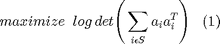
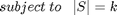
Where S is the optimization variable which contains m possible measurements. Equation (1) can then be re-written in terms of an optimization problem (2):

The solution to (2) is the theoretical 'most optimum point', which can be denoted as  . Given that this problem is a Boolean-convex problem, it can be very time consuming and resource heavy to solve. To make it a computationally easier problem to solve, it helps to relax the constraints (i.e. make the constraints convex):
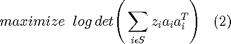

The solution to (3), given the relaxed constraints, is denoted as  . Theoretically, is considered to be an upper bound on , which is the optimal objective value of the original optimization problem (2). Formally, an optimality gap can now be formulated as:
Finally, the problem that the authors seek to solve can be formulated - given that and can be found, is there a method to optimize so that the optimality gap can be minimized?
The authors propose a method that involves swapping the sensors that comprise to narrow the optimality gap. Their proposed method will be implemented and tested in the following sections.
Proposed Solution
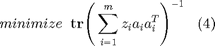
To solve the relaxed constraint cost function (3) in CVX, the solver will attempt to solve the log-determinant function iteratively, which can be very time consuming. To replicate the method the authors used would involve writing a solving routine via Newton's method, which is not the intent of this report. Rather, the goal of this report is to utilize CVX and implememnt novel algorithms. However, the authors do suggest alternative cost functions, one of which is shown in equation (4). This cost function is much faster to solve as it is based on mean squared error, which can be generalized as the trace of the covariance:

The solution can be found by utilizing CVX. Then, sensors that comprise the optimal solution can be swapped and compared with a cost function (5) to see if the optimality gap has been reduced.
![$$S = I + \Big[\begin{matrix} a_j^T\\ a_l^T\\ \end{matrix}\Big]
\hat{\Sigma} \Big[ \begin{matrix} -a_j\ a_l\ \end{matrix}\Big]\;\;\;(5)$$](main_eq99262.png)
Where  is the sensor swapped out, and
  is the sensor that has been swapped in.
The determinant of (5) is taken to see if it is greater than 1; if so, the  is greedily updated as shown in (6), as are the
  values. The equation in (6) is also known as the Woodbury formula.
![$$\hat{\Sigma}=\hat{\Sigma}-\hat{\Sigma}\Big[ \begin{matrix} -a_j\ a_l\
\end{matrix}\Big]S^{-1}
\Big[\begin{matrix} a_j^T\\ a_l^T\\ \end{matrix}\Big]\hat{\Sigma} \;\;\;(6)$$](main_eq89585.png)
This update process for continues until an optimality condition is reached. In simple terms, algorithmically,the flow is as follows:
- Find upper bound, lower bound, and z optimal
- Swap sensors in z optimal with excluded sensors
- Did the swap decrease the cost function? If yes, update z optimal with the swap as well as the covariance metric
- With the new z optimal, re-do the swapping function to see if a better solution can be found (i.e.
 swaps)
 - Continue until there are no more swaps occuring, or the limit of iterations is reached
- Compare the resultant optimality gap as a result of swaps
Data sources
The data used for this implementation is derived from the paper;  sensors with
  parameters to estimate with a
  distribution
clear all

% Data generation occurs in this snippet of code

m = 100;    % number of sensors
n = 20;     % dimension of x to be estimated
kones = ones(1,100);
randn('state', 0);
A = randn(m,n)/sqrt(n);

% end data generation
Solution
[m, n] = size(A);
kstart = 20;
kfin = 45;
i=0;
kappa = log(1.01)*n/m;
onemat = ones(m);
limit = (10*m^3/n^2);


for k=kstart:1:kfin
    i=i+1;


%CVX Optimization begins here
    cvx_begin quiet

    variable z(m,m) semidefinite diagonal
    minimize trace_inv(A'*z*A)

    subject to
        onemat'*z*onemat == k;  %sum of z must equal k (have k sensors)
        1 >= z(m,m) >= 0;

    cvx_end
%CVX Optimization ends here

    z = diag(z,0);
    zsort=sort(z);      %z is sorted highest to lowest
    thres=zsort(m-k);   %treshold can also be arbitrary
    z_star=(z>thres);   %threshold used for rounding values to 1 or 0

    % Swap algorithm

    Low_bound(i) = log(det(A'*diag(z_star)*A));     %Low bound calc
    p_star = z;     %p_star is the theoretical upper bound
    Upp_bound(i) = log(det(A'*diag(p_star)*A)) + 2*m*kappa; %Upper bound calc

    E_hat = inv(A'*diag(z_star)*A); %covariance matrix to be used in swapping alg cost func
    iteration=0;
    numswaps(i)=0;
    while iteration < limit
        swap=0;
        sens = find(z_star==1); no_sense = find(z_star==0);
        for in = sens'
            %look at all chosen sensors
            for out = no_sense'
                %look at all sensors not chosen
                iteration = iteration+1;
                Aj = A(in, :);
                Al = A(out,:);
                S = eye(2)+[Aj; Al]*E_hat*[-Aj' Al'];   %cost function

                if(det(S) > 1)
                    %eval cost function, if greater than 1, do a swap
                    E_hat = E_hat - E_hat*[-Aj' Al']*inv(S)*[Aj; Al]*E_hat;
                    z_star(out) = 1;    %swaping out/in sensor selection
                    z_star(in) = 0;
                    swap=1;
                    numswaps(i) = numswaps(i)+1;
                end

            end
            if swap==1
                break;
            end
        end
        if swap==0
            break;
        end
    end
    z_star2 = z_star;
    Low_bound2(i) = log(det(A'*diag(z_star2)*A));   %lower bound calculation
end
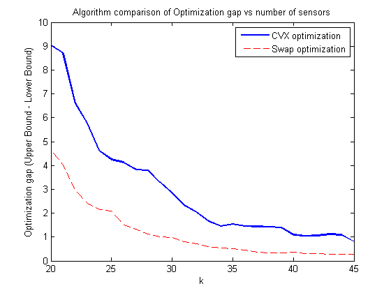
Visualization of results
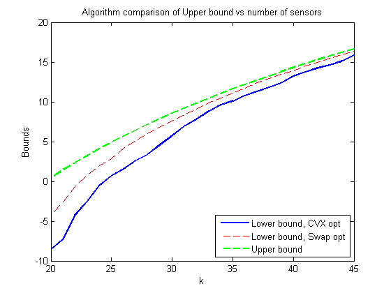
plot(kstart:1:kfin, Upp_bound - Low_bound, 'b', 'LineWidth', 2)
hold on
plot(kstart:1:kfin, Upp_bound - Low_bound2, '--r')
legend('CVX optimization', 'Swap optimization')
xlabel('k')
ylabel('Optimization gap (Upper Bound - Lower Bound)')
title('Algorithm comparison of Optimization gap vs number of sensors')
hold off
figure

plot(kstart:1:kfin, Low_bound, 'b', 'LineWidth', 2)
hold on
plot(kstart:1:kfin, Low_bound2, '--r')
plot(kstart:1:kfin, Upp_bound, '--g', 'LineWidth', 2)
legend('Lower bound, CVX opt', 'Lower bound, Swap opt', 'Upper bound', 'Location', 'SouthEast')
xlabel('k')
ylabel('Bounds')
title('Algorithm comparison of Upper bound vs number of sensors')
hold off

gap1 = Upp_bound-Low_bound;
gap2 = Upp_bound-Low_bound2;

fprintf('Optimality gap vs. Algorithm type\n');
% Where Gap1 represents the CVX optimization as a percentage of the upper
% bound, and Gap2 represents the 'swapping' optimization as a percentage of
% the upper bound.
colLabel = 'Gap1% Gap2% k #Swaps';
iterationLabel = '20 21 22 23 24 25 26 27 28 29 30 31 32 33 34 35 36 37 38 39 40 41 42 43 44 45';
displayMat = [(gap1./Upp_bound.*100)', (gap2./Upp_bound.*100)', (kstart:kfin)', numswaps'];
printmat(displayMat, 'resultstable', iterationLabel, colLabel)
Optimality gap vs. Algorithm type

resultstable =
                     Gap1%        Gap2%            k       #Swaps
           20   2030.11269   1046.93729     20.00000     17.00000
           21    612.80811    282.15588     21.00000     13.00000
           22    280.47687    126.69152     22.00000     21.00000
           23    178.17819     74.23907     23.00000     24.00000
           24    113.04822     52.81843     24.00000     32.00000
           25     86.57224     42.65074     25.00000     20.00000
           26     72.47622     26.40547     26.00000     31.00000
           27     59.24683     20.58909     27.00000     32.00000
           28     52.96512     15.84258     28.00000     34.00000
           29     41.72061     12.69109     29.00000     35.00000
           30     32.96733     11.29026     30.00000     30.00000
           31     25.26395      8.66782     31.00000     25.00000
           32     20.85132      7.41328     32.00000     26.00000
           33     15.86314      5.73150     33.00000     35.00000
           34     13.12514      5.01844     34.00000     26.00000
           35     13.23067      4.31916     35.00000     30.00000
           36     11.88522      3.71346     36.00000     30.00000
           37     11.30635      2.86449     37.00000     33.00000
           38     10.71523      2.63451     38.00000     37.00000
           39     10.11508      2.42011     39.00000     41.00000
           40      7.62463      2.61308     40.00000     40.00000
           41      7.08772      2.01194     41.00000     29.00000
           42      6.96776      1.98211     42.00000     33.00000
           43      7.12046      1.77253     43.00000     32.00000
           44      6.71531      1.63843     44.00000     35.00000
           45      4.82486      1.62914     45.00000     27.00000
Analysis and conclusions
The implementation in this report had a slight difference to the algorithm Joshi & Boyd implemented by utilizing a different cost function; however, the results were identical. The authors were able to get convergence of their swapping implementation at  , which was also demonstrated in this report.
It was found that the swapping optimization algorithm fared much better than non-swapping. Using localized swaps, the algorithm converges much faster to the optimality gap with a reasonable number of swaps (i.e. much less than swaps.
From the results, it is shown that when using the swapping algorithm, getting within 5% of the Upper Limit is possible by selecting sensors; adding additional sensors continues to reduce the gap, and it is shown that the percentage approaches 0 with the higher number of sensors selected.
There is a trade-off with computation speed. The method proposed by the authors is  - therefore for applications such as in real-time computing, it is important to place a limit on iterations or number of sensors to select depending on the final accuracy desired.
Also, there is no clear trend of # of swaps vs. convergence; therefore, although the swap algorithm is , a modest number of swaps will achieve an accurate result.
References
- [1] Joshi, Siddharth, and Stephen Boyd. "Sensor selection via convex optimization." IEEE Transactions on Signal Processing 57.2 (2009): 451-462.
- [2] CVX Research, Inc. CVX: Matlab software for disciplined convex programming, version 2.0. http://cvxr.com/cvx, April 2017
- [3] M. Grant and S. Boyd. Graph implementations for nonsmooth convex programs, Recent Advances in Learning and Control (a tribute to M. Vidyasagar), V. Blondel, S. Boyd, and H. Kimura, editors, pages 95-110, Lecture Notes in Control and Information Sciences, Springer, 2008. https://stanford.edu/~boyd/papers/pdf/graph_dcp.pdf
- [4] Michailovich, O. (2017). ECE 602, Convex Optimization [Lecture notes]. Retrieved from https://ece.uwaterloo.ca/~ece602/outline.html