ECE 602 Project: Multiple Kernel Learning, Conic Duality, and the SMO Algorithm

Problem Formulation
Solution
Data Generation
Primal Problem of SKM
Primal Problem of SKM Which Encourages the Group Sparsity
Dual Problem of SKM
Kernelized Dual Problem of SKM
Results
Conclusions
Reference

Problem Formulation

Classical kernel based classifiers are based on a single kernel, but in practice classifiers based on multiple kernels are more commonly used. The support vector machine (SVM) based on a conic combination of kernels is defined as support kernel machine (SKM). The optimization of the coefficients of such a combination reduces to a convex optimization problem known as a quadratically constrained quadratic program (QCQP). In this project, for the convenience to plot data, we will generate a dataset with two attributes. The whole dataset is divided into two classes with each data point being labeled by 1 or -1. We will first consider the primal and dual problems of SVM, and then the kernelized dual problem will be solved for comparison.

Solution

In linear SVM, the objective is

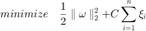
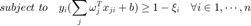
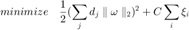
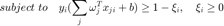
$minimize\quad\frac{1}{2}\parallel \omega\parallel_2^2+C\sum_{i=1}^{n}\xi_i$

$subject\ to \quad y_i(\sum_{j}\omega_j^Tx_{ji}+b)\geq 1-\xi_i \quad\forall i\in {1,\cdots, n}$

In SVM, we encourage the sparsity of the vector $\omega$ at the level of blocks. The primal problem for the SVM is defined as

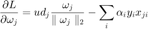
$minimize\quad\frac{1}{2}(\sum_jd_j\parallel\omega\parallel_2)^2+C\sum_i\xi_i$

$subject\ to\quad y_i(\sum_j\omega_j^Tx_{ji}+b)\geq 1-\xi_i, \quad\xi_i\geq 0$

The Lagrangian is

$L=\frac{1}{2}(\sum_jd_j\parallel \omega\parallel_2)^2+C\sum_i\xi_i-\sum_i\alpha_i[y_i(\sum_j^Tx_{ji}+b)-1+\xi_i]-\sum_i\beta_i\xi_i$

When $\omega_j\neq 0$ , $L$ is differentiable, we have

$\frac{\partial L}{\partial\omega_j}=ud_j\frac{\omega_j}{\parallel\omega_j\parallel_2}-\sum_i\alpha_iy_ix_{ji}$

where $u=\sum_jd_j\parallel\omega_j\parallel_2$ . At the minimum, $\frac{\partial L}{\partial\omega_j}=0$ , we have

$ud_j\frac{\omega_j}{\parallel\omega_j\parallel_2}=\sum_i\alpha_iy_ix_{ji}$

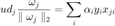
Multiply both sides by $\omega_j^T$ , we have

$ud_j\parallel\omega_j\parallel_2=\omega_j^T\sum_i\alpha_iy_ix_{ji}$

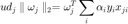
Take the $l_2$ norm of both sides, we have

$ud_j=\parallel\sum_i\alpha_iy_ix_{ji}\parallel_2$

Thus, the Lagrange dual function is

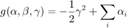
$g(\alpha, \beta, \gamma)=-\frac{1}{2}\gamma^2+\sum_i\alpha_i$

Lagrange dual problem becomes

$maximize\quad -\frac{1}{2}\gamma^2+e^T\alpha$

$subject\ to\quad 0\leq\alpha\leq C,\quad\alpha^Ty=0,\quad\parallel\sum_i\alpha_iy_ix_{ji}\parallel_2\leq d_j\gamma$

We now kernelize the problem using kernel function and get kernelized dual problem.

$minimize\quad\frac{1}{2}\gamma^2-e^T\alpha$

$subject\ to\quad 0\leq\alpha\leq C,\quad\alpha^Ty=0,\quad(\alpha^TD(y)K_jD(y)\alpha)^2\leq\gamma d_j, \forall j$

Data Generation

n = 200;
m = 2;

% Generate 100 points uniformly distributed in the unit disk
r1 = sqrt(rand(n/2,1)); % Radius
t1 = 2*pi*rand(n/2,1);  % Angle
data1 = [r1.*cos(t1), r1.*sin(t1)]; % Points

% Generate 100 points uniformly distributed in the annulus
r2 = sqrt(3*rand(n/2,1)+1); % Radius
t2 = 2*pi*rand(n/2,1);      % Angle
data2 = [r2.*cos(t2), r2.*sin(t2)]; % points

% Put the data in one matrix, and make a vector of classifications
X = [data1;data2];
Y = ones(n,1);
Y(1:n/2) = -1;

rp = randperm(n);
X = X(rp,:);
Y = Y(rp,:);

Primal Problem of SKM

The optimal values of the primal and dual problems should be equal according to strong duality. We can use this property to verify the correctness of the dual probem.

C = 1;

cvx_begin
    variables w(m) xi(n) b;  % w: 34*1, xi: 300*1, b: 1*1
%     dual variable alpha;
    minimize(1/2*w'*w+C*sum(xi));
    subject to
        Y.*(X*w+b)-1+xi >= 0;
        xi >= 0;
cvx_end

 
Calling SDPT3 4.0: 405 variables, 201 equality constraints
------------------------------------------------------------

 num. of constraints = 201
 dim. of socp   var  =  4,   num. of socp blk  =  1
 dim. of linear var  = 400
 dim. of free   var  =  1
 *** convert ublk to linear blk
********************************************************************************************
   SDPT3: homogeneous self-dual path-following algorithms
********************************************************************************************
 version  predcorr  gam  expon
    NT      1      0.000   1
it pstep dstep pinfeas dinfeas  gap     mean(obj)    cputime    kap   tau    theta
--------------------------------------------------------------------------------------------
 0|0.000|0.000|7.1e+00|5.1e+00|4.1e+02| 1.003991e+02| 0:0:00|4.1e+02|1.0e+00|1.0e+00| chol 1   1
 1|0.988|0.988|1.5e+00|1.1e+00|1.5e+02| 2.030366e+02| 0:0:00|3.2e+01|9.4e-01|2.0e-01| chol 1   1
 2|0.889|0.889|5.5e-01|3.9e-01|5.8e+01| 1.865515e+02| 0:0:00|1.9e+00|1.0e+00|7.7e-02| chol 1   1
 3|1.000|1.000|1.9e-01|1.3e-01|2.1e+01| 1.852634e+02| 0:0:00|1.2e-01|1.0e+00|2.7e-02| chol 1   1
 4|0.981|0.981|3.8e-02|2.8e-02|4.2e+00| 1.851030e+02| 0:0:00|5.3e-02|1.0e+00|5.4e-03| chol 1   1
 5|0.781|0.781|2.3e-02|1.7e-02|2.6e+00| 1.852033e+02| 0:0:00|2.0e-02|1.0e+00|3.3e-03| chol 1   1
 6|0.823|0.823|6.2e-03|5.7e-03|6.9e-01| 1.853253e+02| 0:0:00|8.8e-03|1.0e+00|8.9e-04| chol 1   1
 7|1.000|1.000|2.5e-03|2.8e-03|3.0e-01| 1.853529e+02| 0:0:00|1.7e-03|1.0e+00|3.7e-04| chol 1   1
 8|0.921|0.921|2.3e-04|6.1e-04|2.9e-02| 1.853777e+02| 0:0:00|8.4e-04|1.0e+00|3.3e-05| chol 1   1
 9|0.962|0.962|1.0e-05|1.8e-04|1.3e-03| 1.853797e+02| 0:0:00|1.0e-04|1.0e+00|1.5e-06| chol 1   1
10|0.988|0.988|1.7e-07|6.8e-05|1.9e-05| 1.853796e+02| 0:0:00|4.7e-06|1.0e+00|2.4e-08| chol 1   1
11|1.000|1.000|9.9e-09|1.3e-05|1.2e-06| 1.853795e+02| 0:0:00|6.0e-08|1.0e+00|1.4e-09| chol 1   1
12|1.000|1.000|1.5e-09|2.7e-06|1.2e-07| 1.853795e+02| 0:0:00|3.1e-09|1.0e+00|1.1e-10| chol 1   1
13|1.000|1.000|5.9e-09|5.4e-07|1.5e-08| 1.853795e+02| 0:0:00|3.1e-10|1.0e+00|0.0e+00| chol 1   1
14|0.999|0.999|1.3e-09|5.8e-09|3.4e-10| 1.853795e+02| 0:0:00|3.8e-11|1.0e+00|0.0e+00|
  Stop: max(relative gap,infeasibilities) < 1.49e-08
-------------------------------------------------------------------
 number of iterations   = 14
 primal objective value =  1.85379477e+02
 dual   objective value =  1.85379477e+02
 gap := trace(XZ)       = 3.36e-10
 relative gap           = 1.80e-12
 actual relative gap    = -1.08e-10
 rel. primal infeas     = 1.30e-09
 rel. dual   infeas     = 5.83e-09
 norm(X), norm(y), norm(Z) = 1.7e+01, 1.4e+01, 1.4e+01
 norm(A), norm(b), norm(C) = 4.3e+01, 1.4e+01, 1.4e+01
 Total CPU time (secs)  = 0.19  
 CPU time per iteration = 0.01  
 termination code       =  0
 DIMACS: 1.3e-09  0.0e+00  5.8e-09  0.0e+00  -1.1e-10  9.0e-13
-------------------------------------------------------------------
 
------------------------------------------------------------
Status: Solved
Optimal value (cvx_optval): +186.379

Primal Problem of SKM Which Encourages the Group Sparsity

cvx_begin
    variables w2(m) xi2(n) b2;  % w: 34*1, xi: 300*1, b: 1*1
    SUM = norm(w2(1),2);
    for j=2:m
        SUM = SUM+norm(w2(j),2);
    end

    minimize(0.5*SUM^2+C*sum(xi2));
    subject to
        Y.*(X*w2+b2)-1+xi2 >= 0;
        xi2 >= 0;
cvx_end

 
Calling SDPT3 4.0: 409 variables, 202 equality constraints
------------------------------------------------------------

 num. of constraints = 202
 dim. of socp   var  =  3,   num. of socp blk  =  1
 dim. of linear var  = 405
 dim. of free   var  =  1
 *** convert ublk to linear blk
********************************************************************************************
   SDPT3: homogeneous self-dual path-following algorithms
********************************************************************************************
 version  predcorr  gam  expon
    NT      1      0.000   1
it pstep dstep pinfeas dinfeas  gap     mean(obj)    cputime    kap   tau    theta
--------------------------------------------------------------------------------------------
 0|0.000|0.000|7.4e+00|7.4e+00|4.1e+02| 1.002223e+02| 0:0:00|4.1e+02|1.0e+00|1.0e+00| chol 1   1
 1|1.000|1.000|1.8e+00|1.8e+00|1.8e+02| 2.057158e+02| 0:0:00|3.2e+01|9.3e-01|2.2e-01| chol 1   1
 2|0.766|0.766|6.4e-01|6.4e-01|6.3e+01| 1.899186e+02| 0:0:00|5.8e+00|9.9e-01|8.5e-02| chol 1   1
 3|0.959|0.959|2.3e-01|2.3e-01|2.5e+01| 1.853436e+02| 0:0:00|2.6e-01|1.0e+00|3.2e-02| chol 1   1
 4|1.000|1.000|9.2e-02|9.3e-02|1.0e+01| 1.852573e+02| 0:0:00|6.1e-02|1.0e+00|1.3e-02| chol 1   1
 5|0.942|0.942|2.6e-02|2.7e-02|2.8e+00| 1.853844e+02| 0:0:00|2.7e-02|1.0e+00|3.6e-03| chol 1   1
 6|1.000|1.000|1.2e-02|1.3e-02|1.3e+00| 1.854674e+02| 0:0:00|7.0e-03|1.0e+00|1.6e-03| chol 1   1
 7|0.876|0.876|2.6e-03|4.8e-03|2.8e-01| 1.855461e+02| 0:0:00|3.6e-03|1.0e+00|3.6e-04| chol 1   1
 8|0.962|0.962|4.9e-04|1.8e-03|5.9e-02| 1.855631e+02| 0:0:00|8.2e-04|1.0e+00|6.8e-05| chol 1   1
 9|0.978|0.978|1.4e-05|5.7e-04|1.6e-03| 1.855674e+02| 0:0:00|1.6e-04|1.0e+00|1.9e-06| chol 1   1
10|0.989|0.989|2.2e-07|2.2e-04|2.3e-05| 1.855672e+02| 0:0:00|6.1e-06|1.0e+00|3.0e-08| chol 1   1
11|1.000|1.000|1.5e-08|8.7e-05|1.7e-06| 1.855670e+02| 0:0:00|7.2e-08|1.0e+00|2.0e-09| chol 1   1
12|1.000|1.000|1.4e-09|1.7e-05|1.6e-07| 1.855669e+02| 0:0:00|4.4e-09|1.0e+00|1.8e-10| chol 1   1
13|1.000|1.000|2.3e-10|3.5e-07|4.6e-09| 1.855669e+02| 0:0:00|4.1e-10|1.0e+00|1.8e-12| chol 1   1
14|0.999|0.999|1.3e-09|3.8e-09|9.6e-11| 1.855669e+02| 0:0:00|1.3e-11|1.0e+00|0.0e+00|
  Stop: max(relative gap,infeasibilities) < 1.49e-08
-------------------------------------------------------------------
 number of iterations   = 14
 primal objective value =  1.85566889e+02
 dual   objective value =  1.85566889e+02
 gap := trace(XZ)       = 9.60e-11
 relative gap           = 5.15e-13
 actual relative gap    = -8.26e-11
 rel. primal infeas     = 1.33e-09
 rel. dual   infeas     = 3.79e-09
 norm(X), norm(y), norm(Z) = 1.7e+01, 1.4e+01, 1.4e+01
 norm(A), norm(b), norm(C) = 3.9e+01, 1.4e+01, 1.4e+01
 Total CPU time (secs)  = 0.20  
 CPU time per iteration = 0.01  
 termination code       =  0
 DIMACS: 1.3e-09  0.0e+00  3.8e-09  0.0e+00  -8.3e-11  2.6e-13
-------------------------------------------------------------------
 
------------------------------------------------------------
Status: Solved
Optimal value (cvx_optval): +186.567

Dual Problem of SKM

e = ones(n,1);
cvx_begin
    variables gama alpha(n);
    dual variables eq ie;
    maximize(-1/2*gama^2+alpha'*e);
    subject to
        ie : alpha >= 0;
        alpha <= C;
        eq : alpha'*Y == 0;
        SUM = alpha(1)*Y(1)*X(1,:);
        for i = 2:n
            SUM = SUM+alpha(i)*Y(i)*X(i,:);
        end
        norm(SUM,2) <= gama;
cvx_end

 
Calling SDPT3 4.0: 406 variables, 205 equality constraints
------------------------------------------------------------

 num. of constraints = 205
 dim. of socp   var  =  6,   num. of socp blk  =  2
 dim. of linear var  = 400
*******************************************************************
   SDPT3: Infeasible path-following algorithms
*******************************************************************
 version  predcorr  gam  expon  scale_data
    NT      1      0.000   1        0    
it pstep dstep pinfeas dinfeas  gap      prim-obj      dual-obj    cputime
-------------------------------------------------------------------
 0|0.000|0.000|6.6e+01|2.7e+01|2.4e+05|-5.998775e+03  0.000000e+00| 0:0:00| chol  1  1 
 1|0.978|1.000|1.4e+00|3.0e-01|8.9e+03|-2.319266e+02 -3.937326e+03| 0:0:00| chol  1  1 
 2|0.937|0.822|9.2e-02|7.8e-02|2.4e+03|-1.101978e+02 -2.265405e+03| 0:0:00| chol  1  1 
 3|1.000|1.000|2.6e-07|2.1e-02|4.7e+02|-1.094129e+02 -5.720033e+02| 0:0:00| chol  1  1 
 4|0.959|0.879|2.5e-08|2.8e-03|6.2e+01|-1.452422e+02 -2.072103e+02| 0:0:00| chol  1  1 
 5|0.871|0.734|3.1e-08|7.8e-04|1.7e+01|-1.793208e+02 -1.966315e+02| 0:0:00| chol  1  1 
 6|0.646|0.848|1.7e-08|1.2e-04|1.1e+01|-1.814924e+02 -1.921843e+02| 0:0:00| chol  1  1 
 7|0.627|1.000|6.7e-09|3.0e-07|6.2e+00|-1.832276e+02 -1.893922e+02| 0:0:00| chol  1  1 
 8|0.902|1.000|8.6e-10|3.1e-08|2.7e+00|-1.850714e+02 -1.877893e+02| 0:0:00| chol  1  1 
 9|1.000|0.872|6.5e-11|6.8e-09|5.1e-01|-1.862093e+02 -1.867196e+02| 0:0:00| chol  1  1 
10|1.000|1.000|6.0e-16|3.1e-10|1.1e-01|-1.863239e+02 -1.864383e+02| 0:0:00| chol  1  1 
11|0.997|0.909|3.7e-15|5.7e-11|8.3e-03|-1.863779e+02 -1.863862e+02| 0:0:00| chol  1  1 
12|0.984|0.983|3.3e-14|2.0e-12|1.4e-04|-1.863795e+02 -1.863796e+02| 0:0:00| chol  1  1 
13|1.000|0.992|4.3e-14|1.0e-12|2.8e-06|-1.863795e+02 -1.863795e+02| 0:0:00|
  stop: max(relative gap, infeasibilities) < 1.49e-08
-------------------------------------------------------------------
 number of iterations   = 13
 primal objective value = -1.86379476e+02
 dual   objective value = -1.86379479e+02
 gap := trace(XZ)       = 2.80e-06
 relative gap           = 7.50e-09
 actual relative gap    = 7.50e-09
 rel. primal infeas (scaled problem)   = 4.32e-14
 rel. dual     "        "       "      = 1.01e-12
 rel. primal infeas (unscaled problem) = 0.00e+00
 rel. dual     "        "       "      = 0.00e+00
 norm(X), norm(y), norm(Z) = 1.4e+01, 1.7e+01, 1.7e+01
 norm(A), norm(b), norm(C) = 3.1e+01, 1.5e+01, 1.5e+01
 Total CPU time (secs)  = 0.12  
 CPU time per iteration = 0.01  
 termination code       =  0
 DIMACS: 3.3e-13  0.0e+00  7.7e-12  0.0e+00  7.5e-09  7.5e-09
-------------------------------------------------------------------
 
------------------------------------------------------------
Status: Solved
Optimal value (cvx_optval): +186.379

As can be seen from the optimization results, the optimal values of primal problems are equal to that of the dual problem, which proves that the implementation is correct.

Calculate the variables in the primal problem.

w3 = X'*(Y.*alpha);
b3 = -eq;

xt = linspace(min(X(:,1)),max(X(:,1)),n);
yt = -(xt'*w3(1)+b3)/w3(2);

Kernelized Dual Problem of SKM

Generate multiple kernels.

function d=sqdist(a,b)

aa = sum(a.*a,1);

bb = sum(b.*b,1);

ab = a'*b;

d = abs(repmat(aa',[1 size(bb,2)]) + repmat(bb,[size(aa,2) 1]) - 2*ab);

num_kernels=2;
kernel_list=zeros(n*num_kernels,n);
arg_list = [1:num_kernels];
idx_list = zeros(1,1);
for i=1:num_kernels-1,
    idx_list(end+1,:) = floor(m/num_kernels)*i;
end
idx_list(end+1,:) = m;

for i=1:size(idx_list)-1,
    X_temp = X(:,idx_list(i,1)+1:idx_list(i+1,1));
    K = exp(-0.5/i*sqdist(X_temp',X_temp'));
    kernel_list(((i-1)*n+1):(i*n),:)=K;
end

Diganol_Y=diag(Y);

% Use cvx to solve the dual variables.
alpha2=zeros(n,1);
cvx_begin
    variables gamma2 alpha2(n,1);
    minimize(0.5*gamma2^2-sum(alpha2))
    subject to
        alpha2>=0;
        alpha2<=C;
        alpha2'*Y==0;
        for i=1:num_kernels,
            alpha2'*Diganol_Y*kernel_list(((i-1)*n+1):(i*n),:)*...
                Diganol_Y*alpha2<=gamma2;
        end
cvx_end

% Calculate primal variables.
w_phi = 0;  % calculate w*phi
for i=1:n,
    for j=1:size(idx_list)-1,
        X_temp = X(:,idx_list(j,1)+1:idx_list(j+1,1));
        w_phi = w_phi+1/num_kernels*alpha2(i,1)*Y(i,1)*exp(-0.5/j*sqdist(X_temp',X_temp(i,:)'));
    end
end

idx_bias = find((alpha2>0.01)&(alpha2<0.99));  % calculate bias
b_k = Y(idx_bias,:)-w_phi(idx_bias,:);
bias = mean(b_k);
predict = w_phi + bias;
preidct_label = sign(predict);

% Calculate the percentage of correct prediction.
corr=sum(preidct_label==Y)/size(Y,1);

 
Calling SDPT3 4.0: 436 variables, 235 equality constraints
------------------------------------------------------------

 num. of constraints = 235
 dim. of socp   var  = 36,   num. of socp blk  =  3
 dim. of linear var  = 400
*******************************************************************
   SDPT3: Infeasible path-following algorithms
*******************************************************************
 version  predcorr  gam  expon  scale_data
    NT      1      0.000   1        0    
it pstep dstep pinfeas dinfeas  gap      prim-obj      dual-obj    cputime
-------------------------------------------------------------------
 0|0.000|0.000|6.1e+01|2.7e+01|2.4e+05|-5.998775e+03  0.000000e+00| 0:0:00| chol  1  1 
 1|0.792|0.997|1.3e+01|3.7e-01|6.4e+04|-1.289947e+03 -4.836369e+03| 0:0:00| chol  1  1 
 2|0.784|0.629|2.7e+00|1.6e-01|2.1e+04|-2.608089e+02 -5.626658e+03| 0:0:00| chol  1  1 
 3|0.393|0.524|1.7e+00|7.6e-02|1.5e+04|-1.391274e+02 -5.195931e+03| 0:0:00| chol  1  1 
 4|0.271|0.352|1.2e+00|4.9e-02|1.3e+04|-5.925593e+01 -5.225178e+03| 0:0:00| chol  1  1 
 5|0.233|0.513|9.3e-01|2.4e-02|1.1e+04| 8.971149e+00 -5.011705e+03| 0:0:00| chol  1  1 
 6|0.226|0.817|7.2e-01|4.4e-03|8.9e+03| 7.983628e+01 -4.146912e+03| 0:0:00| chol  1  1 
 7|1.000|0.713|2.0e-08|1.3e-03|2.0e+03| 1.324783e+02 -1.827032e+03| 0:0:00| chol  1  1 
 8|0.015|0.031|1.9e-08|1.2e-03|2.0e+03| 9.642755e+01 -1.894903e+03| 0:0:00| chol  1  1 
 9|0.062|0.021|1.8e-08|1.2e-03|2.0e+03| 2.054065e+02 -1.840855e+03| 0:0:00| chol  1  1 
10|0.420|0.823|1.0e-08|2.1e-04|1.8e+03| 1.093468e+02 -1.711820e+03| 0:0:00| chol  1  1 
11|1.000|0.261|6.6e-14|1.6e-04|1.6e+03| 1.738530e+02 -1.424526e+03| 0:0:00| chol  1  1 
12|0.875|1.000|1.7e-13|4.0e-12|8.6e+02| 6.748172e+01 -7.906410e+02| 0:0:00| chol  1  1 
13|1.000|0.793|2.2e-14|2.1e-12|5.3e+02| 2.265900e+01 -5.085528e+02| 0:0:00| chol  1  1 
14|1.000|1.000|1.0e-13|1.0e-12|2.0e+02|-4.652997e+00 -2.048578e+02| 0:0:00| chol  1  1 
15|1.000|1.000|5.5e-15|1.0e-12|8.4e+01|-2.073723e+01 -1.045606e+02| 0:0:00| chol  1  1 
16|1.000|0.945|1.0e-14|1.1e-12|2.9e+01|-3.009020e+01 -5.944477e+01| 0:0:00| chol  1  1 
17|0.691|0.914|1.2e-14|1.1e-12|1.7e+01|-3.278010e+01 -4.951793e+01| 0:0:00| chol  1  1 
18|0.579|1.000|6.9e-15|1.0e-12|9.3e+00|-3.465912e+01 -4.398979e+01| 0:0:00| chol  1  1 
19|0.976|1.000|1.7e-14|1.0e-12|3.8e+00|-3.722485e+01 -4.104533e+01| 0:0:00| chol  1  1 
20|1.000|1.000|1.7e-14|1.0e-12|1.4e+00|-3.813207e+01 -3.951557e+01| 0:0:00| chol  1  1 
21|1.000|1.000|2.2e-15|1.0e-12|4.6e-01|-3.852942e+01 -3.898756e+01| 0:0:00| chol  1  1 
22|0.950|0.904|2.9e-14|1.1e-12|3.8e-02|-3.872699e+01 -3.876485e+01| 0:0:00| chol  1  1 
23|1.000|0.868|2.8e-14|1.1e-12|1.5e-02|-3.873319e+01 -3.874817e+01| 0:0:00| chol  1  1 
24|0.910|0.950|5.6e-14|1.1e-12|3.5e-03|-3.873748e+01 -3.874101e+01| 0:0:00| chol  1  1 
25|1.000|0.962|7.6e-14|1.0e-12|1.2e-03|-3.873864e+01 -3.873988e+01| 0:0:00| chol  1  1 
26|0.952|0.942|1.8e-13|1.1e-12|1.4e-04|-3.873915e+01 -3.873929e+01| 0:0:00| chol  1  1 
27|1.000|1.000|2.0e-12|1.0e-12|2.8e-05|-3.873920e+01 -3.873923e+01| 0:0:00| chol  1  1 
28|1.000|1.000|5.7e-13|1.0e-12|1.1e-06|-3.873921e+01 -3.873922e+01| 0:0:00|
  stop: max(relative gap, infeasibilities) < 1.49e-08
-------------------------------------------------------------------
 number of iterations   = 28
 primal objective value = -3.87392144e+01
 dual   objective value = -3.87392155e+01
 gap := trace(XZ)       = 1.07e-06
 relative gap           = 1.36e-08
 actual relative gap    = 1.36e-08
 rel. primal infeas (scaled problem)   = 5.75e-13
 rel. dual     "        "       "      = 1.00e-12
 rel. primal infeas (unscaled problem) = 0.00e+00
 rel. dual     "        "       "      = 0.00e+00
 norm(X), norm(y), norm(Z) = 1.8e+01, 4.0e+01, 5.8e+01
 norm(A), norm(b), norm(C) = 3.3e+01, 1.5e+01, 1.5e+01
 Total CPU time (secs)  = 0.23  
 CPU time per iteration = 0.01  
 termination code       =  0
 DIMACS: 4.4e-12  0.0e+00  7.6e-12  0.0e+00  1.4e-08  1.4e-08
-------------------------------------------------------------------
 
------------------------------------------------------------
Status: Solved
Optimal value (cvx_optval): -38.7392

Results

Plot the data points and the decision boundary for a linear SVM classifier.

figure(1)
plot(X(find(Y==-1),1), X(find(Y==-1),2),'.r','MarkerSize',10);
hold on
plot(X(find(Y==1),1), X(find(Y==1),2),'.b','MarkerSize',10);
axis equal
plot(xt,yt,'k','LineWidth',1);
hold off
legend('Class A','Class B','Decision Boundary');
title('Linear SVM Classifier');

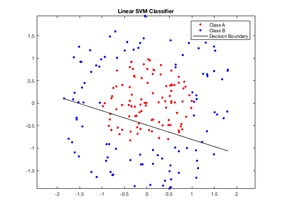
As can be seen from the figure above, when the data has complex distribution, the linear classifier fails to classify two classes. We need to map the data to a higher dimensional space and then apply the linear classifier in the high dimensional space. However, this process can be simplified by a kernel function. The result is shown below.

figure(2)
plot(X(Y==1,1),X(Y==1,2),'.b','MarkerSize',10);
hold on
plot(X(Y==-1,1),X(Y==-1,2),'.r','MarkerSize',10);

d = 0.02;
[x1Grid,x2Grid] = meshgrid(min(X(:,1)):d:max(X(:,1)),...
    min(X(:,2)):d:max(X(:,2)));
xGrid = [x1Grid(:),x2Grid(:)];
d = 0.02;
[x1Grid,x2Grid] = meshgrid(min(X(:,1)):d:max(X(:,1)),...
    min(X(:,2)):d:max(X(:,2)));
xGrid = [x1Grid(:),x2Grid(:)];

kernel_train_test = zeros(size(xGrid,1), size(X,1));
for i=1:size(idx_list)-1,
    X_temp = X(:,idx_list(i,1)+1:idx_list(i+1,1));
    Grid_temp = xGrid(:,idx_list(i,1)+1:idx_list(i+1,1));
    K = 1/num_kernels*exp(-0.5/i*sqdist(Grid_temp',X_temp'));
    kernel_train_test = K + kernel_train_test;
end

prediction_test=kernel_train_test*(alpha2.*Y)+bias;
contour(x1Grid,x2Grid,reshape(prediction_test,size(x1Grid)),[0 0],'k');
legend('Class A','Class B','Decision Boundary');
title('SKM Classifier with Multiple Kernels');
hold off

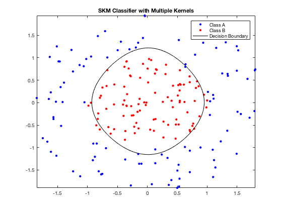
As shown in the figure, SKM yields a better classification boundary for nonlinear cases.

Conclusions

In the original paper[1], F. R. Bach et al. compared the computational complexity of SKM problem based on sequential minimization optimization (SMO) and Mosek. In this project, we generated our own data instead of using real-life data in the original paper. We did not take running time into consideration, but compared the performance of linear SVM with that of SKM with multiple kernels. Using a conic combination of kernels, the classification problem is considered as QCQP, and thus can be solved by CVX. As can be seen from the results:

The optimal values of the primal and dual problems are identical, which means we have solved both problems correctly.

SKM presents a better performance for nonlinear cases.

Reference

[1]Bach, Francis R., Gert RG Lanckriet, and Michael I. Jordan. "Multiple kernel learning, conic duality, and the SMO algorithm." Proceedings of the twenty-first international conference on Machine learning. ACM, 2004.