Introduction

The following report summarizes and implements the technique described in the paper "Time-Optimal Path Tracking for Robots: A Convex Optimization Approach"[1]. The main goal of time-optimal path tracking is to generate a sequence of control inputs that guide the robot (typically a manipulator robot) along some desired path in the least amount of time possible. A simple example would be a robot arm drawing a shape on a piece of paper.

Problem Formulation
Proposed Solution
Data Sources
Solution
Set up robot model matrices for path
Convex problem on page 2323
Plot for different gamma 2
Visualization of Results
Create plot to show energy - time tradeoff
Analysis and Conclusions
References
Appendix

Problem Formulation

This paper employs the decoupled approach to the general problem of time-optimal motion planning. The decoupled approach divides the problem into two sub-problems: path planning and path tracking. The focus of this paper is path tracking and will utilize pregenerated paths in implementation. In general, the time-optimal path will be constrained by the physical properties of the robot such as max motor torque ratings, weights of components, etc.

Original Problem Formulation

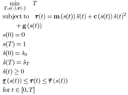
An n-DOF robotic manipulator has joint angles $q$ and joint torques $\tau$ . A path is defined as $q(s)$ which is a function of path coordinate $s$ . $s$ is a function of t; $s(t)$ . The original optimization shown below minimizes the total time $T$ subject to the motion model of the manipulator, start condition, finish condition, and max/min torques of the actuators.

Proposed Solution

Reformulation as a Second Order Cone Program via Direct Transcription

The original problem is reformulated several times to achieve its final form. The details of these reformulations can be seen in the paper and will only be summarized here. First, a convex optimization problem is created based off of the original problem. The objective function is expanded to minimize thermal energy and the integral of the absolute value of the rate of change of the torque. This convex optimization problem is then reformulated using direct transcription to form a large sparse optimization problem. Then finally, the problem is reformulated one last time in order to fit into the form of a second order cone program. The resulting SOCP is shown below.

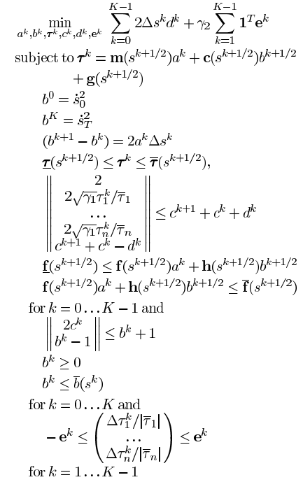
Where

$\tau$ = Joint torques
= Scalar path coordinate
= $\ddot{s}$
= $\dot{s}^2$
= Auxiliary variables from SOCP reformulation
= Acceleration constraints
= $\ddot{q}(s)$
= Index of path element

Data Sources

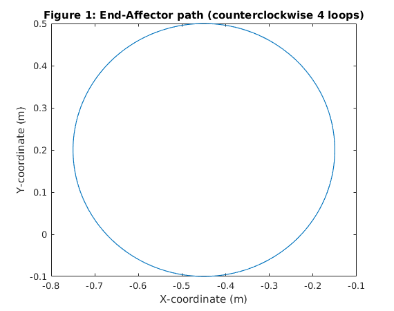
The input to a path tracking algorithm is simply a desired path. In order to stay consistent with the paper, a 2D path was chosen and placed on a plane in 3D space. The Figure below shows the path used to test the proposed solution.

The path was generated using the following code. It samples a circle, producing a discretized series of points.

clc; clear;
run('rvctools/startup_rvc.m');
samples = 600;
radius = 0.3;
centre = [-0.45, 0.2];
cycles = 4;
rad = linspace(0,cycles*4*pi, samples);
x_cir = radius*cos(rad) + centre(1);
y_cir = radius*sin(rad) + centre(2);
figure(3);
clf;
path_x = x_cir;
path_y = y_cir;
plot(path_x, path_y);
xlabel('X-coordinate (m)');
ylabel('Y-coordinate (m)');
title('Figure 1: End-Affector path (counterclockwise 4 loops)');

Robotics, Vision & Control: (c) Peter Corke 1992-2011 http://www.petercorke.com
- Robotics Toolbox for Matlab (release 9.10)
 - pHRIWARE (release 1.1): pHRIWARE is Copyrighted by Bryan Moutrie (2013-2017) (c)
Run rtbdemo to explore the toolbox

Solution

In order to solve the proposed optimization problem numerically, two major pieces of existing software were used.

1. The first is a MATLAB-based robotics toolbox developed by Peter Corke [2]. The toolbox provides a variety of useful functions and object classes to work with various types of robots. The portion that was used for this project was the "mdl_puma560" which is a model of a Puma 560 manipulator robot. The Puma 560 is a 6-DOF manipulator very similar to the KUKA 361 model that was used in the original paper. Inverse kinematics was used to convert the path coordinates into joint angle coordinates. The series of joint angle coordinates is the 'path' used as an input to the optimization problem.

Set up robot model matrices for path

mdl_puma560
T = zeros(4,4,size(path_x,2));
for i=1:size(path_x,2)
    T(:,:,i) = eye(4);
    T(1:3,4,i) = [path_x(i) path_y(i) 0];
end

% now solve the inverse kinematics

q = p560.ikine6s(T);

In addition to inverse kinematics, the Puma 560 model was used to generate matrices that describe the physical properties of the robot such as the inertia matrix, coriolis matrix, gravity loading, and joint friction effects [2]. These matrices were calculated for every point along the path.

s = linspace(0, 1, length(q)+1);
ds = s(2) - s(1);
dqds = [0 0 0 0 0 0;
    diff(q, 1, 1)]/ds;
f = dqds;

d2qds2 = [0 0 0 0 0 0;
    diff(dqds, 1, 1)]/ds;

h = d2qds2;

% Can now calculate mass, coriolis, and grav matrices in terms of path
% coordinates s.
ms = zeros(6, length(q));
cs = zeros(6, length(q));
gs = zeros(6, length(q));
for i= 1:length(q)
    ms(:,i) = p560.cinertia(q(i,:)) * dqds(i,:)';
    cs(:,i) = p560.cinertia(q(i,:)) * d2qds2(i,:)' + ...
        p560.coriolis(q(i,:), dqds(i,:)) * dqds(i,:)';
    gs(:,i) = p560.friction(dqds(i,:)) + p560.gravload(q(i,:));
end

2. The second is CVX which is a convex optimization modelling system based in MatLab [3],[4]. Using CVX, the optimization problem was modelled in MatLab and is shown below. The entire optimization was performed several times with varying values of gamma1 in order to illustrate the trade-off between time-optimality and energy-optimality.

Convex problem on page 2323

set constant torque limit for all the joints

TauMax = 40000*ones(6,length(q));
TauMin = -TauMax;
% Choose a limit for joint acceleration
fmax = [5000 5000 5000 5000 5000 5000];
fmin = -fmax;
% Choose a limit for path velocity
bmax = 500;
% Choose weights for gam1 and gam2 (penalizes thermal energy and rate of
% change of the torques
gam1 = 0;
gam2 = 0;

k = length(q);
n = 6;
cvx_begin quiet
    variable a(k)
    variable b(k+1)
    variable tau1(n,k)
    variable c(k+1)
    variable d(k)
    variable e(k-1)
    % constraints written in paper as being for 0 to k-1 (here is 1 to k)
    for i=1:k
        tau1(:,i) == ms(:,i)*a(i) + cs(:,i)*(b(i+1) + b(i))/2 + gs(:,i);
        c(i+1) + c(i) + d(i) >= norm([2; 2*sqrt(gam1)*(tau1(:,i)./TauMax(:,i)); c(i+1) + c(i) - d(i)]);
        fmin <= f(i,:).*a(i) + h(i,:).*(b(i+1)+b(i))./2;
        fmax >= f(i,:).*a(i) + h(i,:).*(b(i+1)+b(i))./2;
    end
    b(1) == 0;
    b(k+1) == 0;
    b(2:end) - b(1:end-1) == 2*a.*(s(2:end)-s(1:end-1))';
    tau1 <= TauMax;
    tau1 >= TauMin;
    % constraints written for 0 to K (here is 1 to k+1)
    for i=1:(k+1)
        b(i) + 1 >= norm([2*c(i), b(i) -1]);
    end
    b >= 0;
    b <= ones(k+1,1)*bmax;
    % constraints written for 1 to k-1 (here is 2 to k)
    -e <= min((tau1(:,2:end)-tau1(:,1:end-1))./TauMax(:,2:end), [], 1)';
    e >= max((tau1(:,2:end)-tau1(:,1:end-1))./TauMax(:,2:end), [], 1)';
    minimize(2*sum((s(2:end)-s(1:end-1))'.*d) + gam2*sum(e));
cvx_end

Plot for different gamma 2

gam2 = 0.01;
k = length(q);
n = 6;
cvx_begin quiet
    variable a(k)
    variable b(k+1)
    variable tau2(n,k)
    variable c(k+1)
    variable d(k)
    variable e(k-1)
    % constraints written in paper as being for 0 to k-1 (here is 1 to k)
    for i=1:k
        tau2(:,i) == ms(:,i)*a(i) + cs(:,i)*(b(i+1) + b(i))/2 + gs(:,i);
        c(i+1) + c(i) + d(i) >= norm([2; 2*sqrt(gam1)*(tau2(:,i)./TauMax(:,i)); c(i+1) + c(i) - d(i)]);
        fmin <= f(i,:).*a(i) + h(i,:).*(b(i+1)+b(i))./2;
        fmax >= f(i,:).*a(i) + h(i,:).*(b(i+1)+b(i))./2;
    end
    b(1) == 0;
    b(k+1) == 0;
    b(2:end) - b(1:end-1) == 2*a.*(s(2:end)-s(1:end-1))';
    tau2 <= TauMax;
    tau2 >= TauMin;
    % constraints written for 0 to K (here is 1 to k+1)
    for i=1:(k+1)
        b(i) + 1 >= norm([2*c(i), b(i) -1]);
    end
    b >= 0;
    b <= ones(k+1,1)*bmax;
    % constraints written for 1 to k-1 (here is 2 to k)
    -e <= min((tau2(:,2:end)-tau2(:,1:end-1))./TauMax(:,2:end), [], 1)';
    e >= max((tau2(:,2:end)-tau2(:,1:end-1))./TauMax(:,2:end), [], 1)';
    minimize(2*sum((s(2:end)-s(1:end-1))'.*d) + gam2*sum(e));
cvx_end

Visualization of Results

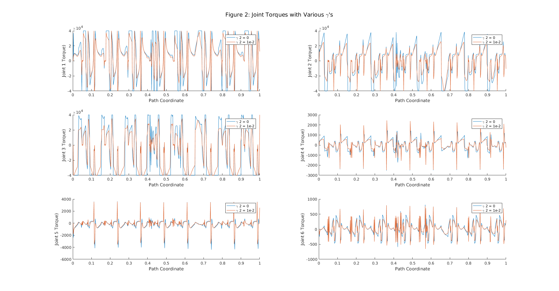
t = cumsum((s(2)-s(1))./sqrt(b(2:end-1)));  %dels is a constant
figure(2);
clf;

subplot(3,2,1);
hold on;
plot(s(2:end), tau1(1,:));
plot(s(2:end), tau2(1,:));
xlabel('Path Coordinate');
ylabel('Joint 1 Torque)');
legend('{\gamma} 2 = 0', '{\gamma} 2 = 1e-2');
subplot(3,2,2);
hold on;
plot(s(2:end), tau1(2,:));
plot(s(2:end), tau2(2,:));
xlabel('Path Coordinate');
ylabel('Joint 2 Torque)');
legend('{\gamma} 2 = 0', '{\gamma} 2 = 1e-2');
subplot(3,2,3);
hold on;
plot(s(2:end), tau1(3,:));
plot(s(2:end), tau2(3,:));
xlabel('Path Coordinate');
ylabel('Joint 3 Torque)');
legend('{\gamma} 2 = 0', '{\gamma} 2 = 1e-2');
subplot(3,2,4);
hold on;
plot(s(2:end), tau1(4,:));
plot(s(2:end), tau2(4,:));
xlabel('Path Coordinate');
ylabel('Joint 4 Torque)');
legend('{\gamma} 2 = 0', '{\gamma} 2 = 1e-2');
subplot(3,2,5);
hold on;
plot(s(2:end), tau1(5,:));
plot(s(2:end), tau2(5,:));
xlabel('Path Coordinate');
ylabel('Joint 5 Torque)');
legend('{\gamma} 2 = 0', '{\gamma} 2 = 1e-2');
subplot(3,2,6);
hold on;
plot(s(2:end), tau1(6,:));
plot(s(2:end), tau2(6,:));
xlabel('Path Coordinate');
ylabel('Joint 6 Torque)');
legend('{\gamma} 2 = 0', '{\gamma} 2 = 1e-2');
suptitle('Figure 2: Joint Torques with Various {\gamma}''s');

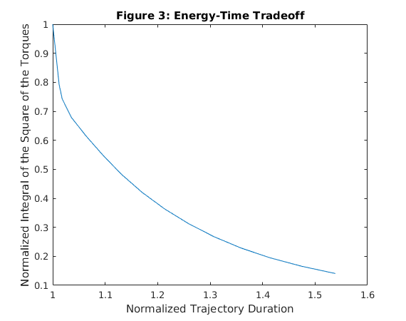
Create plot to show energy - time tradeoff

powers = linspace(-0.9, 0.4, 14);
gammas = 10.^powers;
times = zeros(length(gammas)+1, 1);
energies = zeros(length(gammas)+1, 1);
times(1) = t(end);
energies(1) = sum((tau2(:,1:end-1).^2), 1) * t;

% now just run the optimization a bunch of times
for l=1:length(gammas)
    gam1 = gammas(l);
    cvx_begin quiet
        variable a(k)
        variable b(k+1)
        variable tau(n,k)
        variable c(k+1)
        variable d(k)
        variable e(k-1)
        % constraints written in paper as being for 0 to k-1 (here is 1 to k)
        for i=1:k
            tau(:,i) == ms(:,i)*a(i) + cs(:,i)*(b(i+1) + b(i))/2 + gs(:,i);
            c(i+1) + c(i) + d(i) >= norm([2; 2*sqrt(gam1)*(tau(:,i)./TauMax(:,i)); c(i+1) + c(i) - d(i)]);
            fmin <= f(i,:).*a(i) + h(i,:).*(b(i+1)+b(i))./2;
            fmax >= f(i,:).*a(i) + h(i,:).*(b(i+1)+b(i))./2;
        end
        b(1) == 0;
        b(k+1) == 0;
        b(2:end) - b(1:end-1) == 2*a.*(s(2:end)-s(1:end-1))';
        tau <= TauMax;
        tau >= TauMin;
        % constraints written for 0 to K (here is 1 to k+1)
        for i=1:(k+1)
            b(i) + 1 >= norm([2*c(i), b(i) -1]);
        end
        b >= 0;
        b <= ones(k+1,1)*bmax;
        % constraints written for 1 to k-1 (here is 2 to k)
        -e <= min((tau(:,2:end)-tau(:,1:end-1))./TauMax(:,2:end), [], 1)';
        e >= max((tau(:,2:end)-tau(:,1:end-1))./TauMax(:,2:end), [], 1)';
        minimize(2*sum((s(2:end)-s(1:end-1))'.*d) + gam2*sum(e));
    cvx_end
    temp = cumsum((s(2)-s(1))./sqrt(b(2:end-1)));  %dels is a constant
    times(l+1) = temp(end)'; %Store the time to complete trajectory
    % Calculate the squares of the torque
    energies(l+1) = sum((tau(:,1:end-1).^2), 1) * temp;
end

%Normalize energy and time
times = times./min(times);
energies = energies./max(energies);

figure(3);
clf;
plot(times, energies);
xlabel('Normalized Trajectory Duration');
ylabel('Normalized Integral of the Square of the Torques');
title('Figure 3: Energy-Time Tradeoff');

Analysis and Conclusions

After selecting appropriate constraints for the optimization problem, solutions were obtained with varying values of gamma. The resulting torques calculated via optimization share similar characteristics with torques from the original paper: both display clipping when reaching the torque limit, and increasing {\gamma} 2 results in smoother torques. Also, our torques are periodic which is as expected given that the path is repeating. Figure 3 reproduces the expected trade-off between time-optimality and energy-optimality; matching the result from the original paper. Overall, our results confirm the claims of the original authors stating that their formulation as a convex second order cone program provides a versatile and practical method to path tracking.

References

[1] D. Verscheure, B. Demeulenaere, J. Swevers, J. De Schutter, and M. Diehl, Time-optimal path tracking for robots: A convex optimization approach, IEEE Trans. Automat. Contr., vol. 54, no. 10, pp. 2318-2327, 2009.

[2] P. Corke, Robotics, vision and control: fundamental algorithms in MATLAB. Berlin: Springer, 2013.

[3] Michael Grant and Stephen Boyd. CVX: Matlab software for disciplined convex programming, version 2.0 beta. http://cvxr.com/cvx, September 2013.

[4] Michael Grant and Stephen Boyd. Graph implementations for nonsmooth convex programs, Recent Advances in Learning and Control (a tribute to M. Vidyasagar), V. Blondel, S. Boyd, and H. Kimura, editors, pages 95-110, Lecture Notes in Control and Information Sciences, Springer, 2008. http://stanford.edu/~boyd/graph_dcp.html.

Appendix

The Robotics Toolbox along with the model of the Puma 560 robot was can be found at the following link:

https://github.com/petercorke/robotics-toolbox-matlab

CVX can be found at the following link:

http://cvxr.com/cvx/download/