Face Recognition Based on Image Sets
David Abou Chacra (20581907)
ECE 602 - Winter 2017
Prof. Oleg Michailovich
Paper: Face Recognition Based on Image Sets by Hakan Cevikalp and Bill Triggs [1]
Contents
Problem Formulation and Proposed Solution
The authors describe methods for facial recognition and classification from sets of images, rather than single images. Data in the form of sets of images of individual's faces is usually the output of tracking algorithms run on video streams of different surveillance systems. For example, one or more surveillance cameras track an individual in a certain location from different angles and under varying lighting conditions, and generate a set of images of this individual’s face. The proposed methods allow for utilizing all these facial images to recognize the individual (using a training set of facial images of the individual).
Method Overview
The methods proposed by the authors vary in how their feature space is treated, but follow a general pipeline:
- Every facial image is pre-processed, and has its features extracted (grey-level pixel values, LBP, …etc.).
- Then, every image is treated as a point in n-d space (n being the dimension of the feature vector for a single image).
- A ‘convex shape’ is generated based on the locations of these features.
- The distance between the ‘convex shape’ of the test set, and each of the training sets is computed.
- The test set belongs to the same class as the training set it’s closest to.
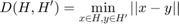
The distance between two convex sets can be seen as the infimum of distances between any point in each of the sets:
Feature Space Parameterization
The authors describe three different methods to parameterize the feature spaces as convex shapes:
1 - Affine Hull: The smallest affine subspace containing the samples. In this space, any affine combination of features of an individual’s face is also seen as part of the Affine Hull, which captures all the set information, but at the same time, is susceptible to noise.
For every individual C, the affine hull is:
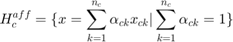
Where  is the kth feature of individual c, and
  is the number of features in the set for individual c.
Using its feature vectors, an affine hull is formulated as:
 :
:
It is parameterized for every individual, C, by:
 : A point that belongs to it (either one of the feature points, a linear combination of two or more of them, and conveniently, the mean of all feature points).
 : An orthonormal basis of the subspace spanned by its feature vectors.
Finding the minimal distance between two affine hulls can be done analytically, as shown in the literature.

Where: U is the orthonormal basis of  and
and  , and
, and 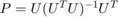 (the orthogonal projection onto the joint span of the two bases).
2 - Reduced Affine Hull: A convex subspace that is between and affine hull and a convex hull in size. It is a tighter convex approximation than an affine hull, which makes it more robust to noise, but it is less restrictive than a convex hull which allows it to describe the data well. The reduced affine hull can actually be formulated as part of a family that includes affine hulls at one extreme and convex hulls at the other extreme, and it is parameterized by an upper and lower bound that determine how tight the boundaries of the convex shape.
Any reduced affine hull can be written, for individual C, as:
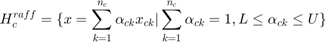
Where  is a vector of coefficients.
In the case of affine hulls  and
and  , meaning the bounds are inactive. Whereas in the case of convex hulls the limits are:
  and
and  which corresponds to the tightest convex boundary around the points (due to the lower bound on alpha being 0). Whereas setting the bounds as :
  and gives a convex shape that is between a convex hull and an affine hull in terms of size, and that is more robust to noise than an affine hull, and less tight than a convex hull. The distance between two reduced affine hulls can be found by solving a constrained optimization problem:


The distance between any two hulls is

Which is the distance between the two closest points in the hulls. This formulation can easily be translated to a cvx optimization problem.
For my numerical solutions, I used the appropriate bounds to parameterize the same reduced affine hull optimization problem, to solve it as an affine hull problem and a convex hull problem.
3 - Convex Hull: As previously stated, the convex hull is the smallest convex shape that contains all the feature points. Setting the bounds in the above formulation to and , allows us to solve for the problem of finding the minimum distance between two convex hulls. In the literature, the problem of finding the minimum distance was replaced by the similar problem of finding a separating hyper plane via a hard-margin SVM formulation. The drawback of this approach is the fact that convex hulls can underestimate the extent of the class if there is a small amount of training data.
In order to reduce noise due to outliers, the authors propose finding a separating hyper plane by solving a soft-margin SVM problem. This is equivalent to setting the bounds as and  . This makes the convex hull reject outliers and makes it more robust to noise.
Data sources
The literature tests the proposed solutions on two datasets: Honda/UCSD dataset, and CMU MoBo.
I tested my implementation on the CMU MoBo dataset which consists of 25 individuals filmed doing 4 different activities from 7 different angles (only 4 of which are usable because the other 3 do not show the faces of the individuals). There are 340 images per camera per activity for every individual.
Faces were detected using the Viola-Jones detector, and then changed in size to 40x40 pixels, and histogram equalized, as mentioned in the paper. For my implementation, I used two viola-jones models, one trained on frontal views of faces, and another on profile views to detect the faces. I extracted gray-level features as well as LBP features (as in the literature), however I only used LBP features for testing, as they are more compact, and therefore can be processed faster.
The MoBo dataset is freely availiable, under permission from its authors [2]
I wrote the function Generate_Mobo_Features to extract features from the MoBo dataset.
clear
clc
close all

load('Directories_Mobo');


%% Initialize Face Detector:
% Initialize two detectors, one for front face, one for profile:
VJFrontFaceDetector = vision.CascadeObjectDetector('UseROI',true);
VJProfileFaceDetector = vision.CascadeObjectDetector('ProfileFace','UseROI',true);
% Regions of interest in the 4 camera angles (to reduce computation time):
ROI_Matrix=[73 40 320 200; ...
    100 68 245 209; ...
    126, 62, 256, 220; ...
    93, 11 272 223];


%% Loop Over All Individuals
for i=1:size(IndividualName,1)
    fprintf('Individual %i\n', i)


    %% Loop Over All Actions For Certain Individual:
    for j= 1:size(ActionName,1)
        fprintf('     Action %i\n', j)
        % Feature Length: 1600 x 1 elements
        % Number of Features: 340(Images)*4(Camera Angles)*2(Face Detectors)= 2720 possible features
        gray_features=zeros(1600,2720);
        LBP_features=zeros(256,2720);

        % Features are taken for a whole action subset over all 4 (viable)
        % camera angles:
        feature_idx=1;

        %% Loop Over 4 Camera Angles for Certain Action:
        for jj= 1:size(CameraAngle,1)
            fprintf('           Camera Angle %i\n', jj)

            Image_Names=dir(strcat('./moboJpg/',IndividualName{i},'/',ActionName{j},'/',CameraAngle{jj},'/*.jpg'));

            %% Loop Over All Images For Certain Camera Angle:

            for k= 1:size(Image_Names,1)

                I=imread(strcat('./moboJpg/',IndividualName{i},'/',ActionName{j},'/',CameraAngle{jj},'/',Image_Names(k).name));

                %% 1 - Viola-Jones Face Detection:
                bboxesFront = step(VJFrontFaceDetector, I, ROI_Matrix(jj,:));
                bboxesProfile = step(VJProfileFaceDetector, I, ROI_Matrix(jj,:));

                %DetectedFrontFaces = insertObjectAnnotation(I, 'rectangle', bboxesFront, ['Front Face: ', num2str(feature_idx)] );
                %DetectedProfileFaces = insertObjectAnnotation(I, 'rectangle', bboxesProfile, ['Profile Face: ', num2str(feature_idx)] );
                %imshow([DetectedFrontFaces DetectedProfileFaces],'InitialMagnification',100)


                if(size(bboxesFront,1)>0)

                    %% 2 - Convert Front Faces to Standard Data:
                    % # Converting to grayscale
                    % # Resizing image to 40x40
                    % # Histogram Equalization
                    for l= 1:size(bboxesFront,1);
                        face=histeq(imresize(rgb2gray(I(bboxesFront(l,2):bboxesFront(l,2)+bboxesFront(l,4),bboxesFront(l,1):bboxesFront(l,1)+bboxesFront(l,3),:)), [40 40]));

                        %% 3 - Populate Feature Matrix:
                        % The feature point is simply the resulting gray values. Alternatively LBP
                        % features can be used.
                        gray_image_feature=face(:);
                        LBP_image_feature=lbp(face)';
                        gray_features(:,feature_idx)=gray_image_feature;
                        LBP_features(:,feature_idx)=LBP_image_feature;
                        feature_idx=feature_idx+1;
                    end

                end

                if(size(bboxesProfile,1)>0)

                    %% 2 - Convert Profile Faces to Standard Data:
                    % # Converting to grayscale
                    % # Resizing image to 40x40
                    % # Histogram Equalization
                    for l= 1:size(bboxesProfile,1);
                        face=histeq(imresize(rgb2gray(I(bboxesProfile(l,2):bboxesProfile(l,2)+bboxesProfile(l,4),bboxesProfile(l,1):bboxesProfile(l,1)+bboxesProfile(l,3),:)), [40 40]));

                        %% 3 - Populate Feature Matrix:
                        % The feature point is simply the resulting gray values. Alternatively LBP
                        % features can be used.
                        gray_image_feature=face(:);
                        LBP_image_feature=lbp(face)';
                        gray_features(:,feature_idx)=gray_image_feature;
                        LBP_features(:,feature_idx)=LBP_image_feature;
                        feature_idx=feature_idx+1;
                    end

                end


            end

        end
        gray_features(:,feature_idx:end)=[];
        LBP_features(:,feature_idx:end)=[];
        save(strcat('./moboJpg/',IndividualName{i},'/GREYfeatures/',IndividualName{i},'_',int2str(j)),'gray_features')
        save(strcat('./moboJpg/',IndividualName{i},'/LBPfeatures/',IndividualName{i},'_',int2str(j)),'LBP_features')
    end
    fprintf('\n')
end
Note that I used an external LBP implementation to generate LBP features, since matlab only implemented its LBP extractor in revision 2015b. The implementation was written by Marko Heikkil and Timo Ahonen.
Solution
For my implementation I tested 4 of the variations of the author's proposed solutions:
- Analytical Affine Hull: I tested the analytical solution proposed to find the distance between two affine hulls defined by the span of their feature vectors. I keep eigenvectors corresponding to 98% and 95% of the total energy in the eigenvalue decomposition (I also tested the method without denoising to compare with the numerical result), which reduces errors due to noisy measuerments.
- Numerical Affine Hull: I tested the solution obtained by minimzing the distance between two reduced affine hulls with limits set to and , i.e with inactive bounds on , the coefficient vector. This theoretically is equivalent to the analytical solution, except that it does not de-noise the data first like the analytical approach does.
- Numerical Reduced Affine Hull: I tested the reduced affine hull approach proposed by the authors(which was untested by them). This was done by numerically finding the closest reduced affine hull to the test set by performing the minimization with bounds:
 and
and  .
. - Numerical Convex Hull: I tested the convex hull approach by solving the actual minimization problem, via the reduced affine hull with
 and
and  . This is contrary to the author's approach of solving this via a soft-margin SVM.
 - Author's Affine Hull: Due to discrepancies in my results and those reported by the authors, I also tested the affine hull source code they provide in their paper. I augment their code to use the MoBo data, as their implementation was only tested on artificial data. Their source code was freely availiable via a link provided in the paper. (Link: http://mlcv.ogu.edu.tr/softwareimageset.html).
Due to the lengthy runtime of performing the experiments, they were only repeated once, unlike the original paper where they were repeated 10 times.
CODE BEGINS
clear
clc

load('Directories_Mobo.mat')

% Create a matrix to specify training and testing sets:
% There are 4 sets for evey individual, I will use 1 to train and 3 to
% test:
TrainTestSet=zeros(size(IndividualName,1),4);
for i=1:size(IndividualName,1)
    TrainTestSet(i,:)=randperm(4);
end
Classify Image Sets Based on Minumum Hull Distance:
Affine Hull
Analytical Affine Hull
The problem is solved using the analytical solution derived in the paper. Here I use the following function to find the distance between two affine hulls defined by their feature vectors:
function [ Dist ] = AnalyticalAffHullDist( Xi, Xj)
% AnalyticalAffHullDist Finds shortest distance between two affine hulls
% analytically
%   This method doesn't use CVX, instead it follows the solution presented
%   in the literature which is in fact an analytical solution.
%
%   Inputs:
%   Xi: Feature vector matrix of one set
%   Xj: Feature vector matrix of other set
%
%   Outputs:
%   Dist: The minimal distance between the selected hulls of the input features


%% Parametrize Affine Hulls:

% I must first find orthonormal bases for each of the affine hulls
% described by the feature vectors Xi and Xj.
% Then I can parametrize this affine hull using the orthonormal basis and
% the mean of feature vectors (or any reference vector that belongs to this
% affine hull).

mui=mean(Xi,2);
muj=mean(Xj,2);
energy_percent=0.95;

Ui=findOrthonormalBasis(Xi, mui, energy_percent);
Uj=findOrthonormalBasis(Xj, muj, energy_percent);

% If the 2 hulls do not intersect, this is an analytical solution for
% finding the minimal distance between the two hulls.
U=orth([Ui -Uj]);
P=U*((U'*U)\U');
Dist=norm((eye(size(P,1))-P)*(mui-muj));


    function [U] = findOrthonormalBasis(X, mu, energy_percent)

        % findOrthonormalBasis: Finds an orthonormal basis for the
        % columnspace of X-mu corresponsing to energy_percent of the
        % total energy.
        % As in the literature, I will resort to using SVD to compute the
        % basis, as it allows us to remove directions corresponding to
        % noisy data (using energy_percent), which the Matlab function orth
        % does not have the functionality to do.
        Normalized_X=X-repmat(mu,[1 size(X,2)]);
        [U, S, ~]=svd(Normalized_X);

        total_energy=sum(diag(S));

        energy_index=1;
        partial_energy=S(1,1);

        while(partial_energy/total_energy<energy_percent)
            energy_index=energy_index+1;
            partial_energy=partial_energy+S(energy_index,energy_index);
        end

        U=U(:,1:energy_index);
    end

end
fprintf('Affine Hull (Analytical) Approach:\n')

% AnalyticalAffineHullClass contains the class predicted by finding minimal distance
% between affine hulls described by the feature vectors:
AnalyticalAffineHullClass=zeros(size(IndividualName,1),4);
AnalyticalAffineHullClass(:,1)=[1:size(IndividualName,1)]';


for i=1:size(IndividualName,1)
    fprintf('Individual %i\n', i)

    % Pick the randomly chosen 1st element of TrainTest as the Training
    % set, and the remaining 3 as test sets:
    for j=2:4
        % Xj is the feature set of the test Image set:
        % Load the precomputed features:
        load(strcat('./moboJpg/',IndividualName{i},'/LBPfeatures/',IndividualName{i},'_',int2str(TrainTestSet(i,j))));
        Xj=LBP_features;
        fprintf('     Test Set %i (%i samples).', j-1, size(Xj,2))

        Distances=inf*ones(size(IndividualName,1),1);

        for k=1:size(IndividualName,1)

            % Xk is the feature set of the training Image set:
            % Load the precomputed features (They are always in column 1 of
            % the variable TrainTestSet:
            load(strcat('./moboJpg/',IndividualName{k},'/LBPfeatures/',IndividualName{k},'_',int2str(TrainTestSet(k,1))));
            Xk=LBP_features;

            Distances(k)= AnalyticalAffHullDist(Xk, Xj);
        end

        [~, predictedclass]=min(Distances);
        fprintf(' Predicted class: %i\n', predictedclass)

        AnalyticalAffineHullClass(i,j)=predictedclass;
    end
end
Numerical Affine Hull
The problem is solved using numerical methods based on the minimization derived in the paper. Here I use the following function to find the distance between two affine hulls defined by their feature vectors:
function [ Dist ] = AffHullDist( Xi, Xj)
%AffHullDist Finds shortest distance between two affine hulls numerically
%using CVX
%   This function was initially the same as Hull Distance(where the values
%   of L and U define what type of hull the feature vectors describe).
%   In the case of a full affine hull: L=-inf , U=+inf.
%   In other words, the bounds are inactive. They were removed to make this
%   function more efficient for CVX to solve.
%
%   Inputs:
%   Xi: Feature vector matrix of one set
%   Xj: Feature vector matrix of other set
%
%   Outputs:
%   Dist: The minimal distance between the selected hulls of the input features


size_ai=size(Xi,2);
size_aj=size(Xj,2);

cvx_begin quiet
% Variables: ai, aj
    variable ai(size_ai,1)
    variable aj(size_aj,1)

    minimize norm(Xi*ai - Xj*aj)

    subject to
        sum(ai)==1;
        sum(aj)==1;
cvx_end

Dist=cvx_optval;

end
fprintf('\nAffine Hull (Numerical) Approach:\n')

% NumericalAffineHullClass contains the class predicted by finding minimal distance
% between affine hulls described by the feature vectors:
NumericalAffineHullClass=zeros(size(IndividualName,1),4);
NumericalAffineHullClass(:,1)=[1:size(IndividualName,1)]';


for i=1:size(IndividualName,1)
    fprintf('Individual %i\n', i)

    % Pick the randomly chosen 1st element of TrainTest as the Training
    % set, and the remaining 3 as test sets:
    for j=2:4
        % Xj is the feature set of the test Image set:
        % Load the precomputed features:
        load(strcat('./moboJpg/',IndividualName{i},'/LBPfeatures/',IndividualName{i},'_',int2str(TrainTestSet(i,j))));
        Xj=LBP_features;
        fprintf('     Test Set %i (%i samples).', j-1, size(Xj,2))

        Distances=inf*ones(size(IndividualName,1),1);

        for k=1:size(IndividualName,1)

            % Xk is the feature set of the training Image set:
            % Load the precomputed features (They are always in column 1 of
            % the variable TrainTestSet:
            load(strcat('./moboJpg/',IndividualName{k},'/LBPfeatures/',IndividualName{k},'_',int2str(TrainTestSet(k,1))));
            Xk=LBP_features;

            Distances(k)= AffHullDist(Xk, Xj);
        end

        [~, predictedclass]=min(Distances);
        fprintf(' Predicted class: %i\n', predictedclass)

        NumericalAffineHullClass(i,j)=predictedclass;
    end
end
Authors Affine Hull
I utilize the implementation supplied by the authors to compare the performance of my implementation to theirs on this specific data. The functions compute_subspace_basis and linear_affinehull_separator were supplied by the authors. It is worth noting that their implementation varies siginificantly from what is mentioned in the paper, and they follow a largely different approach to finding the bases of feature vectors. The link to their implementation: http://mlcv.ogu.edu.tr/softwareimageset.html
fprintf('\nAffine Hull (Authors) Approach:\n')

% NAuthorsAffineHullClass contains the class predicted by finding minimal distance
% between affine hulls described by the feature vectors:
AuthorsAffineHullClass=zeros(size(IndividualName,1),4);
AuthorsAffineHullClass(:,1)=[1:size(IndividualName,1)]';

% The energy threshold (required as input to their function)
th=0.98;

for i=1:size(IndividualName,1)
    fprintf('Individual %i\n', i)

    % Pick the randomly chosen 1st element of TrainTest as the Training
    % set, and the remaining 3 as test sets:
    for j=2:4
        % TestIS is the feature set of the test Image set:

        % Load the precomputed features:
        load(strcat('./moboJpg/',IndividualName{i},'/LBPfeatures/',IndividualName{i},'_',int2str(TrainTestSet(i,j))));
        TestIS=LBP_features;
        fprintf('     Test Set %i (%i samples).', j-1, size(TestIS,2))

        % Find a basis for the subspace spanned by the features:
        [U1, mu1] = compute_subspace_basis(TestIS,'l2',th);

        Distances=inf*ones(size(IndividualName,1),1);

        for k=1:size(IndividualName,1)
            % TrainingIS is the feature set of the training Image set:
            % Load the precomputed features (They are always in column 1 of
            % the variable TrainTestSet:
            load(strcat('./moboJpg/',IndividualName{k},'/LBPfeatures/',IndividualName{k},'_',int2str(TrainTestSet(k,1))));
            TrainingIS=LBP_features;

            % Find a basis for the subspace spanned by the features:
            [U2, mu2] = compute_subspace_basis(TrainingIS,'l2',th);
            [w, b, ad] = linear_affinehull_separator(U1,mu1,U2,mu2); % finding distances between linear affine hulls
            Distances(k)=ad;
        end
        [~, predictedclass]=min(Distances);
        fprintf(' Predicted class: %i\n', predictedclass)

        AuthorsAffineHullClass(i,j)=predictedclass;
    end
end
Reduced Affine Hull
The reduced affine hull problem is solved using cvx based on the minimization derived in the paper. Note that the authors do not report on the results of this formulation, nor do they give any indiciation that they solved it, they merely propose it as a superior method to methods using both affine and convex hull feature spaces. I use the following function to find the distance between two reduced affine hulls defined by their feature vectors, where and :
function [ Dist ] = HullDist( Xi, Xj, L, U)
%HULLDIST Finds shortest distance between two hulls
%   The values of L and U define what type of hull the feature vectors
%   describe.

% In the case of a full affine hull: L=-inf , U=+inf.
% In other words, the bounds are inactive
%
% In the case of a convex hull: L=0, U<1
%
% In the case of a reduced affine hull: L<0 , U>=1
%
%
%
%   Inputs:
%   Xi: Feature vector matrix of one set
%   Xj: Feature vector matrix of other set
%   L: Lower bound of alpha
%   U: Upper bound on alpha
%
%   Outputs:
%   Dist: The minimal distance between the selected hulls of the input features


size_ai=size(Xi,2);
size_aj=size(Xj,2);

cvx_begin quiet
% Variables: ai, aj
    variable ai(size_ai,1)
    variable aj(size_aj,1)

    minimize norm(Xi*ai - Xj*aj)

    subject to
        sum(ai)==1;
        sum(aj)==1;
        ai>=L;
        ai<=U;
        aj>=L;
        aj<=U;
cvx_end

Dist=cvx_optval;

end
fprintf('\nReduced Affine Hull (Numerical) Approach:\n')

% ReducedAffineHullClass contains the class predicted by finding minimal distance
% between affine hulls described by the feature vectors:
ReducedAffineHullClass=zeros(size(IndividualName,1),4);
ReducedAffineHullClass(:,1)=[1:size(IndividualName,1)]';

L=-3;
U=3;

for i=1:size(IndividualName,1)
    fprintf('Individual %i\n', i)

    % Pick the randomly chosen 1st element of TrainTest as the Training
    % set, and the remaining 3 as test sets:
    for j=2:4

        % Xj is the feature set of the test Image set:
        % Load the precomputed features:
        load(strcat('./moboJpg/',IndividualName{i},'/LBPfeatures/',IndividualName{i},'_',int2str(TrainTestSet(i,j))));
        Xj=LBP_features;
        fprintf('     Test Set %i (%i samples).', j-1, size(Xj,2))

        Distances=inf*ones(size(IndividualName,1),1);

        for k=1:size(IndividualName,1)

            % Xk is the feature set of the training Image set:
            % Load the precomputed features (They are always in column 1 of
            % the variable TrainTestSet:
            load(strcat('./moboJpg/',IndividualName{k},'/LBPfeatures/',IndividualName{k},'_',int2str(TrainTestSet(k,1))));
            Xk=LBP_features;

            Distances(k)= HullDist(Xk, Xj, L, U);
        end

        [~, predictedclass]=min(Distances);
        fprintf(' Predicted class: %i\n', predictedclass)

        ReducedAffineHullClass(i,j)=predictedclass;
    end
end
Convex Hull
The convex hull formulation of this problem is solved using cvx also based on the minimization derived in the paper. I use the same HullDist function to find the distance between two convex hulls defined by their feature vectors, where and to reduce suceptibility to outliers:
function [ Dist ] = HullDist( Xi, Xj, L, U)
%HULLDIST Finds shortest distance between two hulls
%   The values of L and U define what type of hull the feature vectors
%   describe.

% In the case of a full affine hull: L=-inf , U=+inf.
% In other words, the bounds are inactive
%
% In the case of a convex hull: L=0, U<1
%
% In the case of a reduced affine hull: L<0 , U>=1
%
%
%
%   Inputs:
%   Xi: Feature vector matrix of one set
%   Xj: Feature vector matrix of other set
%   L: Lower bound of alpha
%   U: Upper bound on alpha
%
%   Outputs:
%   Dist: The minimal distance between the selected hulls of the input features


size_ai=size(Xi,2);
size_aj=size(Xj,2);

cvx_begin quiet
% Variables: ai, aj
    variable ai(size_ai,1)
    variable aj(size_aj,1)

    minimize norm(Xi*ai - Xj*aj)

    subject to
        sum(ai)==1;
        sum(aj)==1;
        ai>=L;
        ai<=U;
        aj>=L;
        aj<=U;
cvx_end

Dist=cvx_optval;

end
fprintf('\nConvex Hull (Numerical) Approach:\n')

% ConxexHullClass contains the class predicted by finding minimal distance
% between affine hulls described by the feature vectors:
ConvexHullClass=zeros(size(IndividualName,1),4);
ConvexHullClass(:,1)=[1:size(IndividualName,1)]';

L=0;
U=0.5;


distcomp.feature( 'LocalUseMpiexec', false )

for i=1:size(IndividualName,1)
    fprintf('Individual %i\n', i)

    % Pick the randomly chosen 1st element of TrainTest as the Training
    % set, and the remaining 3 as test sets:
    for j=2:4
        % Xj is the feature set of the test Image set:
        % Load the precomputed features:
        load(strcat('./moboJpg/',IndividualName{i},'/LBPfeatures/',IndividualName{i},'_',int2str(TrainTestSet(i,j))));
        Xj=LBP_features;
        fprintf('     Test Set %i (%i samples).', j-1, size(Xj,2))

        Distances=inf*ones(size(IndividualName,1),1);

        for k=1:size(IndividualName,1)

            % Xk is the feature set of the training Image set:
            % Load the precomputed features (They are always in column 1 of
            % the variable TrainTestSet:
            load(strcat('./moboJpg/',IndividualName{k},'/LBPfeatures/',IndividualName{k},'_',int2str(TrainTestSet(k,1))));
            Xk=LBP_features;

            Distances(k)= HullDist(Xk, Xj, L, U);
        end

        [~, predictedclass]=min(Distances);
        fprintf(' Predicted class: %i\n', predictedclass)

        ConvexHullClass(i,j)=predictedclass;
    end
end
Results
The results are compared to the known ground truth and stored in the matrix Accuracy_Matrix in the following order:
- Results of modelling features via an Affine Hull and solving analytically.
- Results of modelling features via an Affine Hull and solving numerically.
- Results of modelling features via an Affine Hull and using the author's supplied code.
- Results of modelling features via a Reduced Affine Hull and solving numerically.
- Results of modelling features via a Convex Hull and solving numerically.
The results are as follows:
| Experiment | Our Results | Paper Results |
|---|---|---|
| Linear Affine Hull (Analytical) - Energy Threshold 95% | 84.0% | N/A |
| Linear Affine Hull (Analytical) - Energy Threshold 98% | 72.0% | 94.6% |
| Linear Affine Hull (Analytical) - No Denoising | 60.0% | N/A |
| Linear Affine Hull (Numerical) | 54.7% | 94.6% |
| Linear Affine Hull (Author's Code) | 36.0% | 94.6% |
| Reduced Affine Hull (Numerical) | 66.7% | N/A |
| Convex Hull (Numerical) | 73.3% | 98.1% |
Correct_Class=zeros(size(IndividualName,1),4);

for i=1:size(IndividualName,1)
    Correct_Class(i,:)=i*ones(1,4);
end

Accuracy_Matrix=zeros(5,1);

Accuracy_Matrix(1)=(sum(sum((AnalyticalAffineHullClass-Correct_Class)==0))-size(IndividualName,1))/(size(IndividualName,1)*3);
Accuracy_Matrix(2)=(sum(sum((NumericalAffineHullClass-Correct_Class)==0))-size(IndividualName,1))/(size(IndividualName,1)*3);
Accuracy_Matrix(3)=(sum(sum((AuthorsAffineHullClass-Correct_Class)==0))-size(IndividualName,1))/(size(IndividualName,1)*3);
Accuracy_Matrix(4)=(sum(sum((ReducedAffineHullClass-Correct_Class)==0))-size(IndividualName,1))/(size(IndividualName,1)*3);
Accuracy_Matrix(5)=(sum(sum((ConvexHullClass-Correct_Class)==0))-size(IndividualName,1))/(size(IndividualName,1)*3);
Analysis and Conclusions
Result Discrepancies
The main point to discuss is that the algorithm did not behave at all as expected. While at first I thought this may be a bug in my own code, testing the same data on the author’s code yielded even poorer results far outside the tolerance range proposed in the paper. This discrepancy could have been a result of one or many factors:
- Data differences resulting from the Viola-Jones algorithm: One thing I noted while extracting the data is how poor the performance of the Viola-Jones algorithm was in detecting faces, a lot of the time the faces were missed, and other times erroneous faces were detected that were in fact not faces (mainly background objects). This caused a lot of the individual sets to have very few data samples (7 of the 25 individuals did not have more than 500 out of what should have been 340(Images)*4(Camera Angles)*2(Face Detectors)=2720 features per set). While 5 individuals had a significant portion of their samples corrupted by noise (A background computer that the Viola-Jones algorithm seemed to think was a face across all 5 samples). These samples cannot be considered noise, because they occurred frequently enough, that the algorithm would have considered them part of the main hull, and they definitely confused the closest point algorithm which would confuse these 5 individuals constantly because they essentially contained the same feature cluster in n-d space. This caused 12 out of 24 individuals to have their feature sets be less than ideal. It should be noted that the algorithms mostly failed around these individuals, especially the numerical affine hull, and the author’s affine hull which seemed to be the most susceptible to them.
- Randomness: A less likely cause of the result discrepancy is the randomness in choosing a test and training set, although this doesn’t explain why the author’s code (which was only written to use synthetic data, and I adapted to the MoBo Data) performed so poorly on real data, and did not achieve results remotely within the tolerance described in the paper.
- Data Elimination: In their paper the authors mentioned that they used the data for 24 individuals of the MoBo dataset, while it actually contains 25 individuals, which could indicate they removed one individual entirely before running their tests.
- Algorithm mismatch: The algorithms described in the paper (and the ones I implemented in this project) seemed vastly different from those implemented in the author’s code, which leads me to suspect the author did not publish the finished code for the paper, but rather a first prototype of it.
The most likely cause of the difference in results is the data mismatch. I believe the authors did achieve these numbers on a less noisy, and more 'feature-ful' dataset. The specifics of their implementation of the Viola-Jones algorithm for face detection, or how they generated their dataset are not discussed in the paper, and I could only generate this data at the best of my abilities.
Given this discrepancy, and the obvious effect of noise on the data, I had to decrease the total energy retained by the eigenvalue decomposition to 95% (as opposed to the proposed 98%) in order to get comparable results to those of the paper.
Performance
Despite all the algorithms performing much worse than reported, they, relatively, still performed quite well. Compared to the chance probability of correct classification (100/25=4%), the algorithms all performed significantly better. The analytical affine hull, reduced affine hull and convex hull methods all proved to be good methods, and extremely resilient to noise and outliers (especially given that 50% of the data may have been corrupted by it, as stated earlier). I believe with a better face detection algorithm these methods would perform significantly better and approach the results cited in the paper.
It is interesting to compare the results of the analytical affine hull approach versus the numerical one. The most worthy thing to note is how removing data corresponding to smallest 2% and 5% of the energy (de-noising) caused such an improvement in the performance of the algorithm. Testing the analytical affine hull method while keeping the noisy data (Energy Threshold=100%). Actually gave a comparable result to the numerical affine hull approach which doesn’t remove the noise (60% for the analytical affine hull versus 55% for the numerical approach). This is likely due to the intersection of affine hulls of one or more classes which leads to the shortest distance being 0 for several classes, the output class being essentially a tossup between these erroneous classes.
Applicability
I do not see this method being very applicable outside a theoretical formulation. The method exhibits a lot of drawbacks:
- Susceptibility to noise: I had to severely threshold the energy of the eigenvalue decomposition to get results that are reliable enough, which is a bad indicator of the method’s robustness to noise. It is possible that changing the lower and upper bounds on the convex hull’s approximation would also lead to better results, while the numerical affine hull is essentially a lost cause.
- Runtime: The analytical method is somewhat fast, whereas all the numerical methods are extremely slow. This is due to each numerical method having to solve an optimization problem with 4 * feature-vector length constraints, which amounts to around 1000 constraints while using LBP features, and 6400 constraints when using gray levels. This is in addition to the algorithm having to solve one of these problems for every training set available, in order to find the class to which it has the shortest distance to overall. For a relatively small dataset of 25 people this is still possible, but in case the data size grows, this becomes a more and more complex problem that is being solved very inefficiently.
- Superiority of newer methods: Newer methods like deep networks are capable of solving such problems with ease, and would likely be faster and more accurate than the methods described in this paper.
References
- Cevikalp, Hakan, and Bill Triggs. "Face recognition based on image sets." Computer Vision and Pattern Recognition (CVPR), 2010 IEEE Conference on. IEEE, 2010.
- R.Gross and J. Shi. "The CMU Motion of Body (MoBo) Database" Tech. Report CMU-RI-TR-01-18 Robotics Institute, Carnegie Mellon University, 2001