Distance Metric Learning for Large Margin Nearest Neighbor Classification
ECE 602 Final Project
Alison Cheeseman and Jonah Ho
April 23, 2018
Contents
Introduction & Problem Formulation
The k-nearest neighbours (kNN) rule is one of the simplest methods of pattern classication, however when combined with prior knowledge it can yield comptetive results. The kNN rule classifies unlabeled examples by taking the majority label among its k nearest neighbours in the training set, and thus its performance depends on the distance metric used to identify the nearest neighbours. Ideally, the distance metric used for kNN classification should be chosen to suit the problem at hand, and it has been shown in recent literature that the results can be significantly improved by learning a distance metric from a set of training data.
In this paper, kNN classification is improved by learning a Mahalanobis distance metric which is optimized with the goal that the k nearest neighbours to an example always belong to the same class and examples from different classes are separated by a large margin. This approach is referred to as large margin nearest neighbour (LMNN) classification. The LMNN approach differs from previous approaches in the literature which seek to minimize pairwise distances between all similarly labeled examples.
Proposed Solution
In this section we outline the proposed solution. First, we define the model and some important notation. We let  denote our training set of
  labeled examples with input features
  and discrete labels
  and we define the binary matrix
  to indicate whether the labels and
  match. For each input
  we also specify
  target neighbours, as the nearest neighbours (according to Euclidean distance, which share the same label . We then define a second binary matrix,
  to indicate whether input is a target neighbour of
  .
.
The goal is then to find a linear transformation  which will be used to compute the squared Mahalanobis distance, as follows:
In particular, we want to learn  which will optimize the performance of kNN classification using this distance metric. To do so we define a cost function with two competing terms. The first term penalizes large distances between each input and its target neighbours, while the second term penalizes small distances between each input and all other inputs which do not share it's label by way of the standard hinge loss. The cost function is given by
![$$ \epsilon(L) = \sum_{ij}\eta_{ij}||L(\bar{x_i}-\bar{x_j})||^2 + c\sum_{ijl}\eta_{ij}(1-y_{il})[1 + ||L(\bar{x_i}-\bar{x_j})||^2-||L(\bar{x_i}-\bar{x_l})||^2]_+$$](main_eq15206934702141895973.png)
where  is a constant which gives weight to each term and is typically set by cross validation. The minimization of the above cost function can be reformulated as a semidefinite program (SDP) by noting that

where  is a positive semidefinite matrix. We introduce a slack variable
  to "mimick" the hinge loss for each pair of differently labeled inputs. The resulting SDP is given by


which can be solved using most standard optimization solvers, such as CVX.
Data Sources
For our report we tested the LMNN algorithm on two data sets, all of which are publicly available at http://www.ics.uci.edu/~mlearn/MLRepository.html. The two data sets used are the "Iris" and "Wine" data sets, each of which group the data into three classes. The data was modified so that the class labels are given by  . The code below stores some information about each data set so that we can load them and run the algorithm.
clc;
clear all;
close all;

fname = ["iris_modified","wine_modified"];
N_data = length(fname);
N_features = [4 13];
N_classes = [3 3];
Solution
In this section we present our code to run the LMNN algorithm and compare the results to the standard kNN classification using the Euclidean distance. We use CVX to solve for the optimal matrix  which parameterizes the Mahalanobis distance. Due to time constraints we fix the parameters of the optimization to be
  and
and  , instead of using cross-validation as is done in the original paper.
After the optimal is found we run the kNN classification and LMNN algorithms on each data set. The kNN and LMNN algorithms can be implemented using the built in Matlab function, 'knnsearch' with the standard Euclidean distance, and a custom distance function which implements the Mahalanobis distance with the optimal matrix .
N = 5; % number of experiments
err_e = zeros(N_data,1);
err_m = zeros(N_data,1);

k = 3; % number of nearest neighbours
c = 1; % weight of hinge loss

for n = 1:N_data % loop over each data set
% Here we read in the data set and split it into features (x) and labels
% (y),
fileID = fopen(sprintf('data/%s.data',fname(n)),'r');
formatspec = [repmat('%f,',1,N_features(n)),'%d'];
D = fscanf(fileID,formatspec,[N_features(n)+1,Inf]);
x_in = D(1:N_features(n),:).';
y_in = D(N_features(n)+1,:).';
clear D;

for nn=1:N % loop over each 'experiment'
% Next, the data is randomly split into training (70%) and test (30%) sets.
[x_train,x_test,y_train,y_test] = split_data(x_in,y_in);
N_train = length(y_train);

% Now we solve the convex optimization problem to find the matrix, M.
[eta, x_train, y_train, ~] = generate_eta([x_train y_train], N_train, N_features(n));
y_ij = generate_y_ij(y_train);
% CVX solution goes here.
x = x_train.';
IND = find(eta==1);
[indx1,jndx] = ind2sub(size(eta),IND);
indx1 = indx1.';
jndx = jndx.';
clear IND;

IND = find(y_ij==0);
[indx2,lndx] = ind2sub(size(y_ij),IND);
indx2 = indx2.';
lndx = lndx.';
clear IND;

indx = [];
for m =1:length(indx1)
    kndx = find(indx2==indx1(m));
    indx = [indx; repmat(indx1(m),[size(kndx),1]).' repmat(jndx(m),[size(kndx),1]).' lndx(kndx).'];
end

cvx_begin quiet
    variable M(N_features(n),N_features(n)) symmetric
    variable Xi(length(indx)) nonnegative
    sum_left = 0;
    sum_right = 0;
    for m = 1:length(indx)
        i = indx(m,1);
        j = indx(m,2);
        sum_left = sum_left + ((x(:,i)-x(:,j)).'*M*(x(:,i)-x(:,j)));
        sum_right = sum_right + Xi(m);
    end
    f0 = sum_left + c*sum_right;
    minimize f0
    subject to
    Xi>=0;
    M == semidefinite(N_features(n));
    for m = 1:length(indx)
        i = indx(m,1);
        j = indx(m,2);
        l = indx(m,3);
        (x(:,i)-x(:,l)).'*M*(x(:,i)-x(:,l))-(x(:,i)-x(:,j)).'*M*(x(:,i)-x(:,j)) >= 1-Xi(m);
    end
cvx_end

% Next we implement the kNN algorithm using the proposed Mahalanobis distance
% and the Euclidean distance, for comparison
y_out_e = knn_euclidean(N_classes(n),x_train,y_train,x_test,k); % Euclidean distance
y_out_m = knn_mahalanobis(N_classes(n),x_train,y_train,x_test,k,M); % Mahalanobis Distance

% %  Now we compute the testing error rate.
err_e(n) = err_e(n) + sum(y_out_e~=y_test)/(length(y_test));
err_m(n) = err_m(n) + sum(y_out_m~=y_test)/(length(y_test));
end
end

% % Finally, we average the error rate over N experiments and convert to a percentage.
err_e = (100/N)*err_e;
err_m = (100/N)*err_m;
Visualization of Results
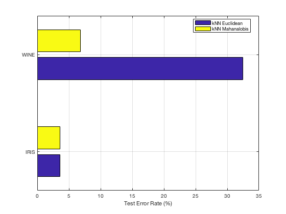
In the following we plot the error rate on the test data, averaged over 5 experiments with different random 70/30 splits of each data set.
c = categorical({'IRIS','WINE'});
E = [err_e(1) err_m(1); err_e(2) err_m(2)];

figure,
barh(E);
grid on;
legend('kNN Euclidean','kNN Mahanalobis','location','best')
set(gca,'yticklabel',char(c));
xlabel('Test Error Rate (%)')
Analysis and Conclusions
Our implementation of the LMNN algorithm appears to have successfully learned an optimal Mahalanobis distance metric for kNN classification. We see in the case of the IRIS data set that there is minimal improvement, which is suspected to be due to overfitting, as is mentioned in the original paper. However, on the WINE data set we observe a significant improvement in performance when we apply our optimized distance function.
Quantitavely, our results differ from those of the original paper as the CVX solution converges slowly for such a high-dimensional problem and this led to time constraints for this project. As a result, we did not implement cross-validation to set the problem parameters k and c, we just used default values. We also only were able to run the experiment 5 times and compute an average error rate, whereas the rates cited in the paper are averaged over 100 experiments.
References
[1] K.Q. Weinberger, J. Blitzer and L.K. Saul, 'Distance Metric Learning for Large Margin Nearest Neighbour Classification', Proc. Advances in Neural Information Processing Systems (NIPS 2005), MIT Press, 2006.
Appendix A: List of Functions
The following custom functions (submitted along with this report) were used in the above implementation:
split_data.m
knn_euclidean.m
knn_mahalanobis.m
mahalanobis_dist.m
generate_eta.m
generate_y_ij.m