Polynomial-Decay Averaging Scheme for SGD: Implementation and Evaluation

A reconstruction of "Stochastic Gradient Descent for Non-smooth Optimization: Convergence Results and Optimal Averaging Schemes"

Submitted as project report for ECE602

Yankun Cao (y243cao@)

1. Problem Formulation
2. Proposed Solution
3. Benchmark Problem (SVM)
4. Our Implementation
5. Experiments and Results
5.1 COV1
5.2 MNIST
6. Conclusion
List of Attached Files
Reference

1. Problem Formulation

Stochastic Gradient Descent (SGD) is an iterative approximation algorithm for solving optimization problems, i.e. minimizing $F(w)$ over $w\in W$ . Its updating algorithm is defined as:

$w_{t+1} = \Pi_W(w_t-\eta_t \hat{g}_t), (1)$

where $w_{t+1}$ , $w_t$ are the intermediate solutions, $w_1$ is an initial guess, $\eta_t$ is a step size parameter, $\hat{g}_t$ is an estimate of a subgradient $g_t\in \partial F(w_t)$ , and $\Pi_W$ denotes the projection onto the feasible set $W$ .

A trivial method of applying this algorithm is to run it for a number of iterations, and take the result from the last iteration ( $w_T$ ) as the solution to the optimization problem. However, as argued in the paper that we studied [1] (we will refer to it as 'the paper' in all following sections), and other work [4] preceding the paper, it is better, in terms of rate of convergence to the optimum, to take a weighted average, $\bar{w}_T$ , of $w_1$ , $w_2$ , ..., $w_T$ as the final solution. Hence, the goal of the paper is to propose a new averaging scheme for calculating $\bar{w}_T$ , and compare it to other schemes.

2. Proposed Solution

The paper presents polynomial-decay averaging:

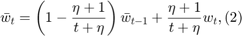
$\bar{w}_t=\left(1-\frac{\eta+1}{t+\eta}\right)\bar{w}_{t-1} +\frac{\eta+1}{t+\eta}w_t, (2)$

where $\eta>0$ is a parameter, and $\bar{w}_1=w_1$ . Note that the parameter $\eta$ is a different variable from the step size parameter $\eta_t$ in formula $(1)$ ; this might be confusing but here we stick with the notation of the paper.

3. Benchmark Problem (SVM)

In this section we describe the benchmark optimization problem for comparing polynomial-decay averaging against other baseline methods. This benchmark problem is used both in the paper and our reconstruction.

The problem is solving SVM, i.e. minimizing the following function:

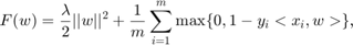
$F(w) = \frac{\lambda}{2}||w||^2+ \frac{1}{m}\sum_{i=1}^{m}\max\{0,1-y_i<x_i,w>\},$

over the variable $w\in \mathbf{R}^d$ , where $\lambda \in \mathbf{R}_+, y_i\in \{-1, 1\}, x_i\in \mathbf{R}^d (i = 1, 2, ..., m)$ are known. For this problem, one closed form solution of the gradient $\hat{g}_t$ is:

$\hat{g}_t = \lambda w_t-\mathbf{1}_{y_i<x_i,w_t>\leq 1}y_i x_i, where\ i\ is\ randomly\ drawn\ from\ \{1, 2, ..., m\},$

so that formula $(1)$ can be calculated. Note that since the domain is $\mathbf{R}^d$ , we can ignore the projection operation in $(1)$ .

Furthermore, the paper sets the initial guess $w_1=0$ , the step size parameter $\eta_t=\frac{1}{t\lambda}$ , and the polynomial-decay averaging parameter $\eta=3$ .

4. Our Implementation

Next we describe how we implement the proposed solution and other baseline methods for comparison, in order to solve the benchmark problem.

Since the proposed solution and the benchmark problem is straight-forward and described in details by the paper, we follow every formula as discussed in the previous sections. We do not make use of external libraries, and use only the basic features provided by MATLAB. To construct similar graphs as the paper, we keep the $(T, F(\bar{w}_T))$ value pairs for a set of different $T$ . Note that for collecting and visualizing results, we output results as raw text to a csv file, and further process/visualize it using Excel (files included in submission). For exact source code and individual comments, please refer to the end of this section.

As for baseline methods for comparison, we pick two other weighted-averaging schemes and implement them as well. Baseline 1 is simple averaging, which is also used in the paper:

$\bar{w}_t = \frac{1}{t}\sum_{i=1}^{t}w_i,$

which can be re-formulated as:

$\bar{w}_t = (1-\frac{1}{t})\bar{w}_{t-1}+\frac{1}{t}w_t.$

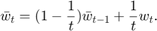
This is in fact exactly the same as formula $(2)$ , if we set the parameter $\eta=0$ , and this is how we implement it. Baseline 2 is just taking the last element: $\bar{w}_t = w_t$ . This is used for comparison in another research paper proposing a different averaging scheme [4], and because it is so simple we also want to test it out.

Note that for the solution proposed by the paper, and the baseline methods we choose, they are all very efficient, in the way that the computation of $\bar{w}_t$ only relies on no more than $\bar{w}_{t-1}$ and $w_t$ , so that they consume minimal constant storage (no need to store $w_1$ to $w_{t-1}$ and $\bar{w}_1$ to $\bar{w}_{t-2}$ once they have been used) and the computation is very simple.

Below is our entire source code. We will continue to describe our dataset and present our experiments after that.

% Pre-defining parameters.
lambda = 0.000001; % 0.000001 for Covertype dataset; 0.01 for MNIST.
ita = 3; % 3 for polynomial-decay averaging (in the paper); 0 for simple averaging (baseline 1).
num_rounds = 2 ^ 15;

% Reading Covertype data.
raw_data = csvread('covtype.data');
[n, m] = size(raw_data); % Should be [581012, 55], second dimension being 54 attributes + 1 label.
                         % Note that in our source code the usage of m and n
                         % is different from the paper; i.e. n is the number
                         % of samples while m is the dimension of vectors.
X = raw_data(:, 1:m-1);

% Normalizing features (optional).
% X = (X - min(X)) ./ (max(X) - min(X));

y_raw = raw_data(:, m); % Labels come in [1, 2, ..., 7], which will be
                        % converted to [1, -1, -1, ..., -1] for our purpose.
twos = ones(n, 1) * 2;
y_interm = min(twos, y_raw); % [1, 2, ..., 7] => [1, 2, 2, ..., 2].
y = 3 - y_interm * 2; % [1, 2] => [1, -1].

w = zeros(m-1, 1);

% Reading MNIST data.
%{
X = csvread('MNIST_X_train.csv'); % This dataset is already normalized to [0, 1].
[n, m] = size(X); % Should be [60000, 784].
y_raw = csvread('MNIST_y_train.csv'); % Labels come in [0, 1, ..., 9], which will be
                                      % converted to [1, -1, -1, ..., -1] for our purpose.
y_interm = min(ones(n, 1), y_raw); % [0, 1, ..., 9] => [0, 1, 1, ..., 1].
y = 1 - y_interm * 2; % [0, 1] => [1, -1].
w = zeros(m, 1);
%}

w_avg = w;
t = 1;
next_t_to_print = t; % Less-printing mode for MUCH better efficiency.

out_file = fopen('out.csv', 'w'); % Preparing output file, for keeping (log2(T), log2(F)) values.

while t <= num_rounds
    %{
    % Always-printing mode. VERY SLOW.
    F = sum(max(zeros(n, 1), ones(n, 1) - y .* (X * w_avg))) / n + (w_avg' * w_avg) * lambda / 2;
    fprintf(out_file, '%f, %f\n', log(t) / log(2), log(F) / log(2)); % Outputting log2(t), log2(F).
    % fprintf('%d/%d\n', t, num_rounds); % Printing progress to console.
    %}

    if t >= next_t_to_print % Less-printing mode.
        next_t_to_print = next_t_to_print * 2; % Only printing at exponents of 2.
        F = sum(max(zeros(n, 1), ones(n, 1) - y .* (X * w_avg))) / n + (w_avg' * w_avg) * lambda / 2;
        fprintf(out_file, '%f, %f\n', log(t) / log(2), log(F) / log(2)); % Outputting log2(t), log2(F).
        % fprintf('%d/%d\n', t, num_rounds); % Printing progress to console.
    end

    % Starting the SGD algorithm in the paper.
    i = randi([1 n]);
    g = lambda * w - (y(i) * X(i, :) * (X(i, :) * w * y(i) <= 1))';
    w = w - (1 / (lambda * t)) * g;
    t = t + 1;

    % The paper: ita = 3; baseline 1: ita = 0;
    w_avg = (1 - (ita + 1) / (ita + t)) * w_avg + ((ita + 1) / (ita + t)) * w;

    % Baseline 2: taking last element.
    % w_avg = w;
end

fclose(out_file);

5. Experiments and Results

We conduct experiments on two datasets: COV1 and MNIST. Below, for each dataset, we will provide an overview of the dataset itself, describe experiment setup, and present results and analysis.

5.1 COV1

Dataset Overview

COV1 is the only dataset used in the paper that is publicly available online. It is an adapted version from the Covertype dataset [2]. Because the original Covertype dataset is a multi-class dataset, while the benchmark problem is for binary classification, a one-versus-rest model is applied to convert it to COV1. Namely, class 1 from the original dataset is still considered as class 1 in COV1, while all other class are converted to be class -1 in COV1.

In the COV1 dataset, there are 581012 samples, each with 54 real-valued attributes (i.e. $x_i\in \mathbf{R}^{54}, m=581012$ ) and a class label of -1 or 1. In total, there are 211840 samples of class 1, and 369172 samples of class -1. For this dataset, the paper sets the parameter $\lambda = 10^{-6}$ .

In the following, we first try to reconstruct the experiment in the paper and produce a similar graph (Experiment 1), and then move on to investigate side issues that we find interesting (Experiment 2 and 3).

Experiment 1: Rate of Convergence

In order to demonstrate that polynomial-decay averaging has a faster rate of convergence, we need to collect value pairs $(T, F(\bar{w}_T))$ as the algorithm progresses, repeat multiple times for more confidence, and plot them on a graph. If, compared to the baselines, polynomial-decay averaging always has a smaller $F(\bar{w}_T)$ at a given $T$ , and, preferably, also smaller variations over the multiple runs, then we can conclude that this method has a faster rate of convergence (and better stability).

To test this, we use our implementation of polynomial-decay averaging and the baseline methods, and apply them to the benchmark optimization problem on the COV1 dataset. We repeat each setup 5 times. Similar to the paper, we only collect a small set of selected $T$ and associated $F(\bar{w}_T)$ values (in log-log scale) for visualization. Our implementation outputs the values as raw text to csv files, and then we use Excel to process and visualize the results.

Figure 1 shows the plot of $(T, F(\bar{w}_T))$ , in log-log scale, with error bars, for 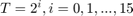$T = 2^i, i = 0, 1, ..., 15$ , for all three algorithms. (If the figure is not clear enough in this html file, please refer to the Excel spreadsheet that is also attached.) Note that the plots always start at $(0, 0)$ , because when $T=1$ , we have $\bar{w}_1=0$ , and $F(0)=1$ , but this trivial solution does not have any practical value in the SVM problem.

From the figure we can see that as T increases, polynomial-decay averaging always produces a smaller $F(\bar{w}_T)$ , and the error bars are also tighter, compared to the baseline methods, so we conclude that the solution proposed by the paper converges faster than the others, and is more stable in the process. This is consistent with the results and the conclusion presented by the paper.

There are some minor issues, though. First, while the simple averaging scheme (baseline 1) performs the worst, taking the last element (baseline 2) seems to provide decent performance compared to polynomial-decay, at least at some point in Figure 1. Hence, we would like to further compare these two in some other way, so that we can fully justify the solution proposed by the paper. This is discussed in the following section (Experiment 2). Second, there is actually one inconsistency between our results and that of the paper, which is the scale of $\log_2 F(\bar{w}_T)$ . In particular, in the paper, that value decreases approximately from 12 to 0, while in our Figure 1 the function value decreases from 43 to around 27. We conjecture that this is due to pre-processing of the dataset that is not mentioned in the paper. To justify our hypothesis, we briefly investigate this issue in Experiment 3.

Experiment 2: Further Comparison

Because in the last experiment, polynomial-decay averaging does not significantly stand out compared to taking the last element, in this section we further compare the two methods in detail to try to decide which method is better and why.

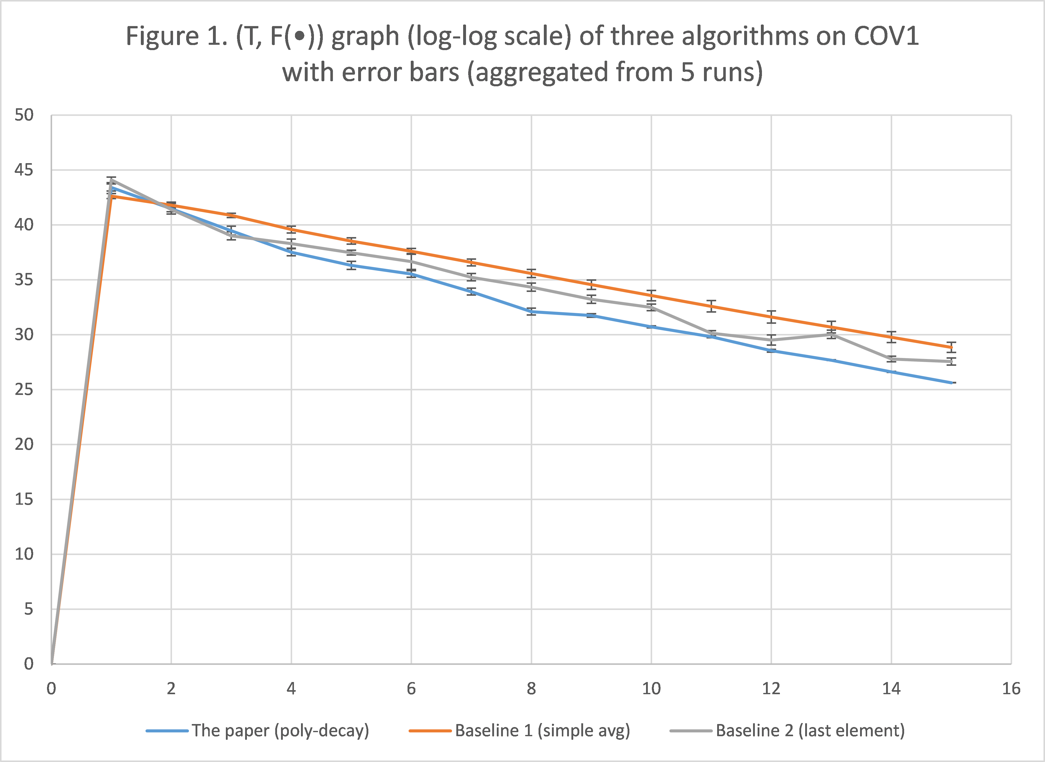
Note that in the last experiment, we only plot the graph where $T$ is an exponent of 2, which is much smaller than the entire set, and only provides a very limited snapshot of the algorithms' behavior. To further study the convergence pattern of the two methods in question, we collect all $(T, F(\bar{w}_T))$ value pairs during a single run, and plot them on graphs. And it turns out that it is exactly in this experiment that the two algorithms start to demonstrate notable difference.

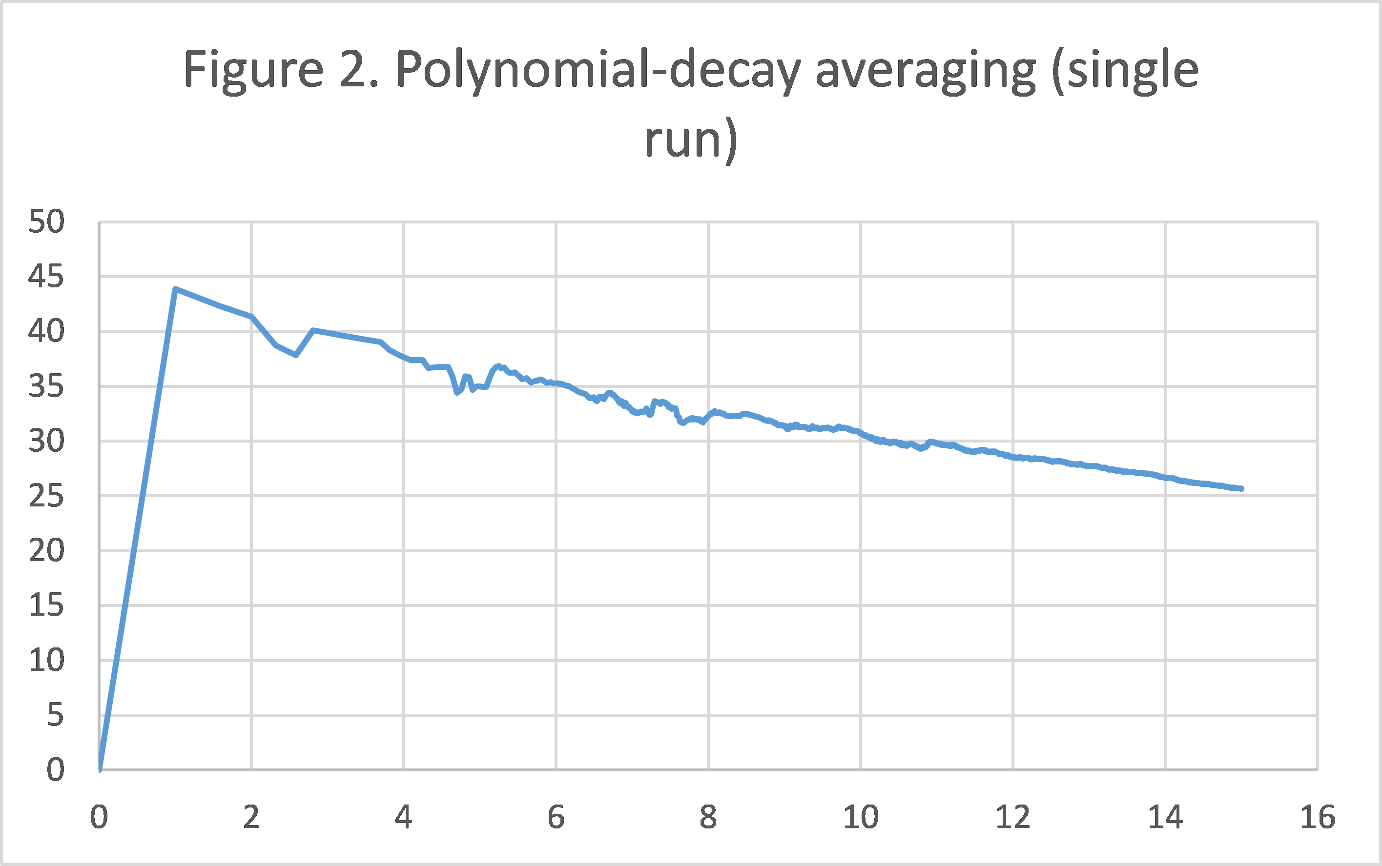
Figure 2/3 shows the convergence pattern of polynomian-decay averaging/taking last element during a single run. As we can see, towards the end of the graph, the method of taking the last element is extremely unstable in terms of objective function value. Meanwhile, the graph of polynomial-decay averaging is very smooth, even though in a log-log scale, there are much more data points packed towards the end.

We believe this suffices to justify the solution proposed by the paper: not only does it converge faster and have a smaller variation for a fixed number of iteration (as shown by the smaller averages and tighter error bars in Experiment 1), it is also much more stable in consecutive rounds during a single run (shown in this experiment).

Experiment 3: The Impact of Pre-processing

Lastly, we try to address the fact that our results have a different magnitude compared to the paper. We speculate that this is due to data pre-processing that is not mentioned in the paper, but still a natural step in taking any problem on real-life data. In particular, we would like to test whether using some trivial data pre-processing can really change the magnitude of the objective function value.

To carry this out, we pre-process the COV1 dataset by normalizing all attributes to the interval [0, 1] (a linear projection from [min, max] to [0, 1]), and apply the polynomial-decay averaging scheme for a single run. We collect results for $T=2^i, i = 0, 1, ..., 25$ , and compare them to those obtained from the original COV1 that is not normalized, in Figure 4.

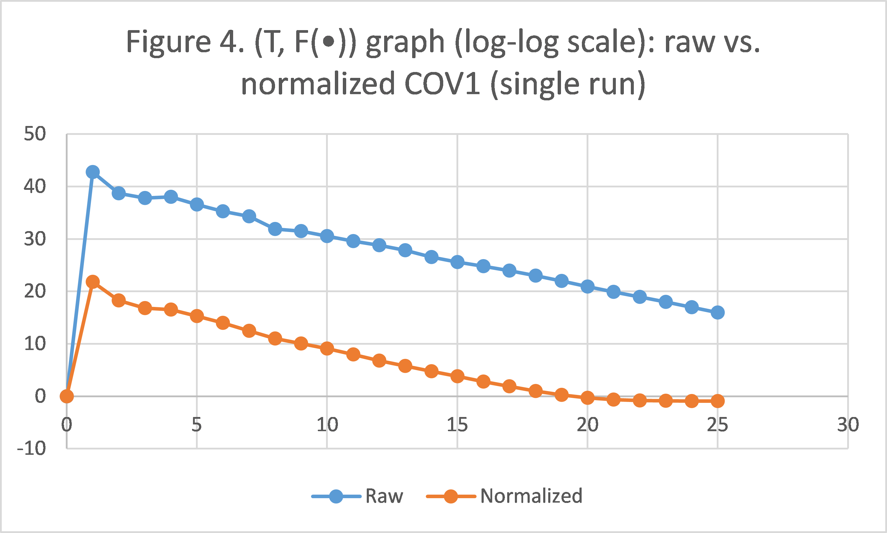
Indeed, having a dataset normalized can significantly impact the objective function value. In our case, results from the normalized COV1 are always smaller by a magnitude of approximately $2^{20}$ , until when $T=2^{21}$ , where the algorithm on the normalized dataset actually converges, while the algorithm on the original COV1 still has a long way to go. This actually gives us some insight if we look at it another way: for optimization problems, applying certain pre-processing techniques may greatly reduce the time needed for SGD with polynomial-decay averaging to reach convergence (as long as the pre-processing techniques make sense in the scope of the optimization problem). As in our case, optimization on the original dataset takes 16 times the running time ( $2^{25}/2^{21}=16$ ), but is still nowhere near convergence.

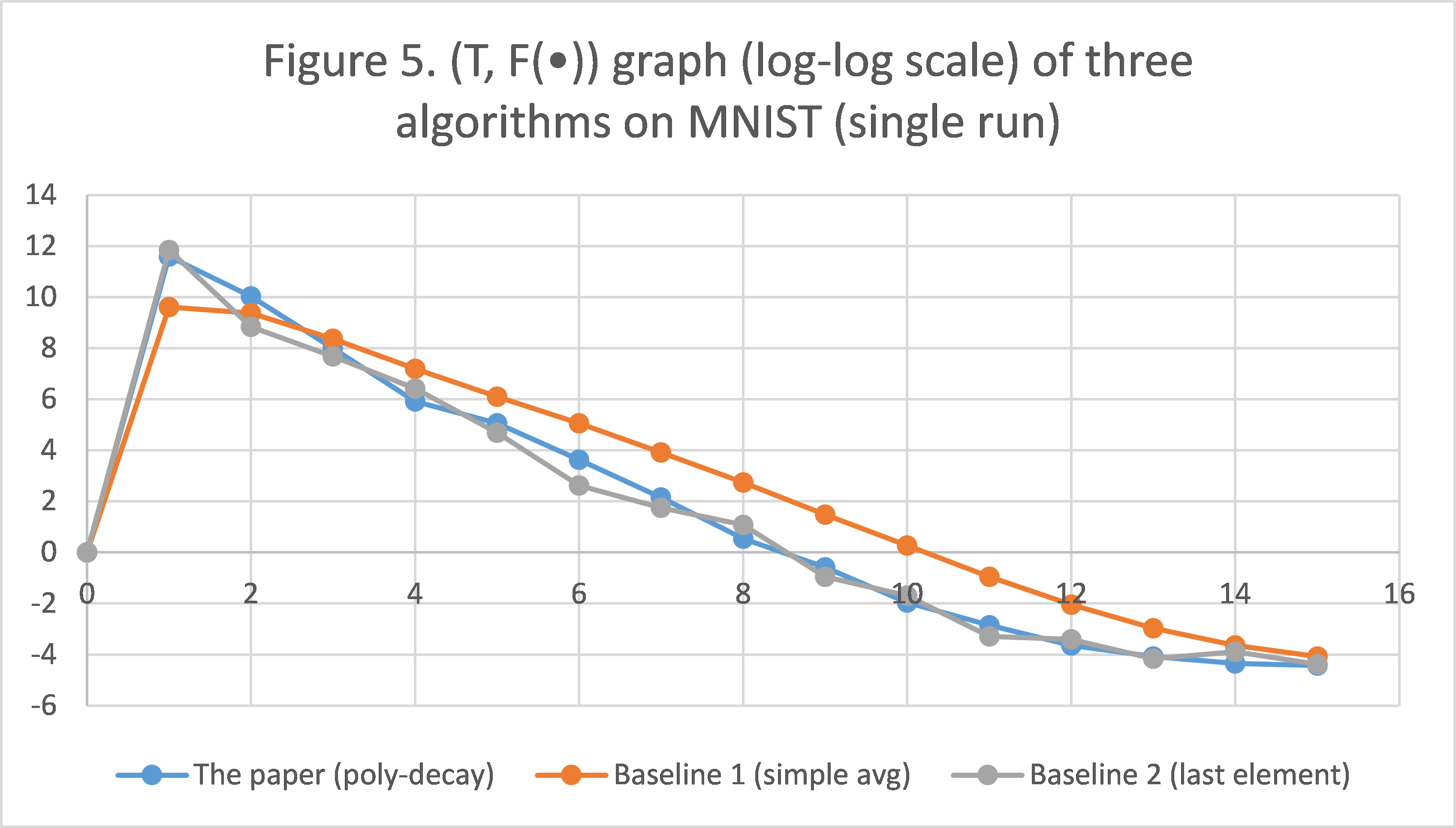
5.2 MNIST

We conduct an additional experiment on the training set of MNIST to compensate for our lack of datasets (since two other datasets used in the paper are not available). We also note that the positive and negative samples are rather balanced in COV1 (211840:369172), so we would like to test our algorithms where the two classes are not balanced, so we chose MNIST and converted it into an unbalanced binary classification problem, which we desribe in the next section.

Dataset Overview

The training set of MNIST [3] contains 60000 samples, each with 784 non-negative attributes and a class label in $\{0, 1, ..., 9\}$ . The ten classes are fairly balanced. To convert it to a binary classification problem, we consider class 0 as positive, and all others as negative, so we have a class ratio of around 1:9. The dataset we use is normalized (all attributes are in [0, 1]). For the parameters, we set $\lambda=10^{-2}$ , while all other parameters are the same as the ones used in the COV1 experiments.

Experiment

We apply the proposed solution and the two baselines for a single run, collect the results, and plot them in Figure 5. Again, simple averaging is underwhelming; taking last element is comparable to polynomial-decay averaging, but is less consistent/stable. This shows that our conclusions still hold when the two classes are unbalanced.

6. Conclusion

In our course project, we implemented the polynomial-decay averaging scheme for SGD, as proposed by the paper we studied [1]. We used our implementation, and compared it to two other baseline methods, simple averaging and taking last element, on the same optimization problem used in the paper. Our results show that the proposed solution converges faster than simple averaging, while being more stable than taking last element, which does not contradict the original paper. As a side observation, we discovered that pre-processing a dataset (such as normalization) can greatly reduce the run time needed to reach convergence.

List of Attached Files

Other than the files required by the course project (main.m and html files), we attach the following files in the folder /Additional_Files for vierwers' reference.

COV1_AllResults.xlsx contains Figures 1 to 4 and all necessary data for plotting the figures.

Directory /COV1_RawOutput contains all the raw csv files generated from Experiments 1 to 3. These results are combined to produce COV1_AllResults.xlsx.

MNIST_Results.xlsx contains Figure 5 and associated data.

src_clean.m is our source code without the text for report generation (but has all comments about the code).

Paper.pdf is the paper.

Reference

[1] O. Shamir and T. Zhang, "Stochastic gradient descent for non-smooth optimization: convergence results and optimal averaging schemes," ICML'13

[2] Covertype dataset: https://archive.ics.uci.edu/ml/datasets/covertype

[3] MNIST dataset: http://yann.lecun.com/exdb/mnist/

[4] A. Rakhlin, O. Shamir and K. Sridharan, "Making gradient descent optimal for strongly convex stochastic optimization," ICML'12