Engine ON/OFF Control for the Energy Management of a Serial Hybrid Electric Bus via Convex Optimization

Contents

Problem Formulation

Energy management problem of engine ON/OFF control of a serial hybrid electric bus.

Proposed Solution

An effective technique consists of splitting the optimization problem into two parts. First part consists of defining an engine ON/OFF strategy, whereas the second part consists of optimizing the power split based on that ON/OFF strategy.

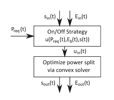
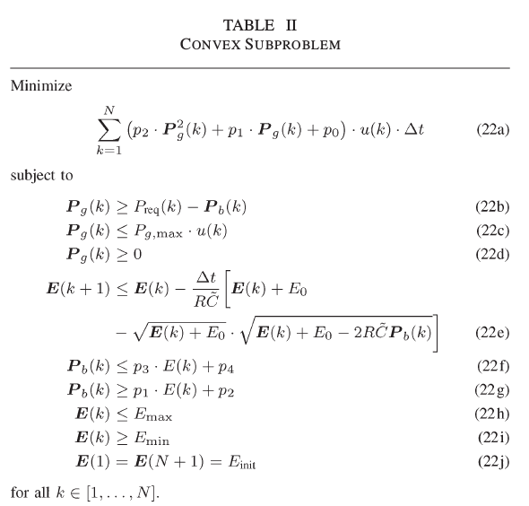
The optimization problem can be formulated as seen in table II. This is the equation that will give us the optimal fuel consumption of the engine subject to generator power constraints, power delivered, and energy content.

Data Sources

The data used in this experiment is randomly generated. The source data is not available in the reading. The only information available in the reading were the constant values.

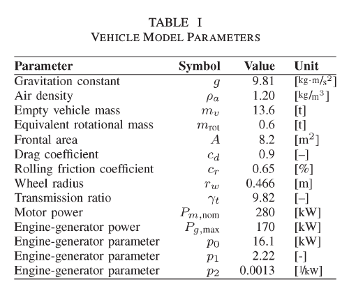
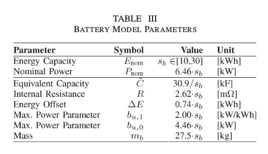
clear
clc

%Constants - Own



i = 0;
N = 1000;

e = zeros(1,2001);
theta_lim = zeros(1,2001);

%Constants - Paper

g = 9.81; %Gravitation constant [kg m/s^2]
pa = 1.20; %Air density [kg/m^3]
mv = 13.6; %Empty vehicle mass [t]
mrot = 0.6; %Equivalent rotational mass
A = 8.2; %Frontal area [m^2]
cd = 0.9; %Drag coefficient [-]
cr = 0.65; %Rolling friction coefficient [%]
rw = 0.466; %Wheel radius [m]
yt = 9.82; %Transmission ratio [-]
Pm_nom = 280; %Motor power [kW]
Pg_max = 170; %Engine-generator power [kW]
p0 = 16.1; %Engine-generator parameter [kW]
p1 = 2.22; %Engine-generator parameter [-]
p2 = 0.0013; %Engine-generator parameter [1/k W]

p3 = 10;
p4 = 10;

C = 30.9;
R = 2.62;
E_delta = 0.74;

e_max = 30;
e_min = 10;
e_init = 20;

Ib = .01;

s = [3,3,3,3,3,3,3];
k = 0.5;


Eo = 0;
Uo = 0;
% Q = linspace(75,25,2001);
Q = (35-30).*rand(2001,1) + 35;
Max_val = (30-20).*rand(1,1) + 30;
Min_val = (12-6).*rand(1,1) + 12;
Range_1 = (300-200).*rand(1,1) + 300;
pg = linspace(Max_val, Min_val ,Range_1);
Min_val = (4-1).*rand(1,1) + 4;
Range_2 = (300-200).*rand(1,1) + 300;
pg2 = linspace(min(pg),Min_val,Range_2);
Max_val = (16-10).*rand(1,1) + 16;
pg3 = linspace(min(pg2),Max_val,(1002-(Range_1 + Range_2)));
pg = [pg,pg2,pg3];

%Variables
Ft = zeros(1,2000); %Required force
Fa = zeros(1,2000); %Aerodynamic drag force
Ff = zeros(1,2000); %Rolling friction force
Fg = zeros(1,2000); %Up/Downhill driving force

m = zeros(1,2000); %mass of the vehicle

Solution

%Iterative solution

for i=1 : N

    if i>=3
      s(i) = s(i-1) + k * (s_out(i-2) - s(i-1));
    elseif i==2
        s(i) = 3;
    elseif i==1
        s(i) = 3;
    end

    %calculate voltage source

    Uoc(i) = (Q(i)/C) + Uo;

    %calculate buffer energy

    e(i) = (1/2) * C * Uoc(i)^2 - Eo;

    %calculate engine on/off

    B(i) = (C*R)/(2*(e(i)+E_delta));


    preq(i) = Pm_nom;

    theta_lim(i) = ((1/2)*(p1 - s(i))+sqrt(p0 * (s(i)*B(i)+p2)))/(s(i)*B(i));


            pb_max(i) = p3*e(i) + p4;
        pb_min(i) = p1*e(i) + p2;


    if theta_lim(i)> pb_max(i)
        plim(i) = pb_max(i);
    elseif theta_lim(i) < pb_min(i)
        plim(i) = pb_min(i);
    else
        plim(i) = theta_lim(i);
    end



    if preq(i) >= plim(i)
       u(i) = 1 ;
    else
        u(i) = 0;
    end

    %calculate power delivered

    pb(i) = Uoc(i) * Ib - R * Ib^2;

    %optimize
    cvx_begin quiet
        minimize ((p2 * pg(i)^2 + p1 * pg(i) + p0) * u(i));
        pg(i) >= preq(i) - pb(i);
        pg(i) <= Pg_max * u(i);
        e(i+1) <= e(i)- (1/R*C)*(e(i)+ Eo - sqrt(e(i)+Eo) * sqrt(e(i) + Eo - 2*R*C*pb(i)));
        pb(i)<=p3*e(i) + p4;
        pb(i)>=p1*e(i) + p2;
        e(i) <= e_max;
        e(i) >= e_min;
        e(1) = e_init;
        e(N+1) = e_init;

    cvx_end

    Pf(i) = cvx_optval;
    temp = ((.0005 +.0025).*rand(1,1) - .0018);
    s_out(i) = s(i) + temp;
end

Visualization of the results

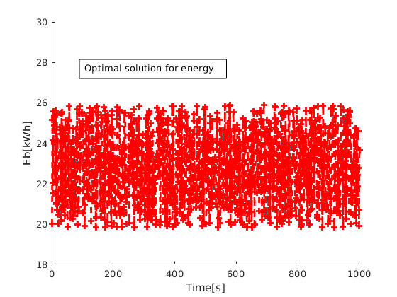
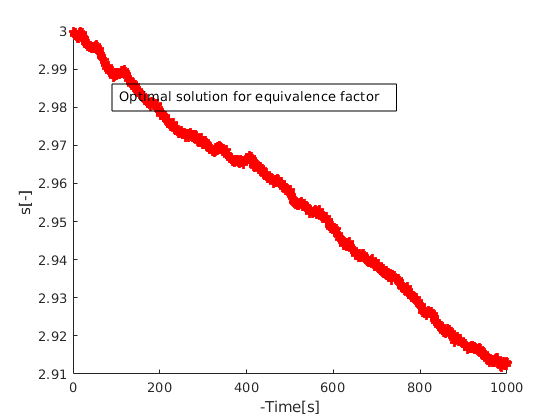
dim = [.2 .5 .3 .3];

figure(1)
hold on
xlabel('Time[s]') % x-axis label
ylabel('Eb[kWh]') % y-axis label
plot(1:N, e(1,1:N),'r+--','Linewidth',2);
annotation('textbox',dim,'String','Optimal solution for energy','FitBoxToText','on');
ylim([18 30])
hold off

figure(2)
hold on
xlabel('Battery Capacity[Wh]') % x-axis label
ylabel('I/100km') % y-axis label
r1=plot(1:N, Pf(1,1:N),'r+--','Linewidth',2);
annotation('textbox',dim,'String','Optimal solution for battery capacity','FitBoxToText','on');
hold off

figure(3)
hold on
xlabel('-Time[s]') % x-axis label
ylabel('s[-]') % y-axis label
r1=plot(1:N, s(1,1:N),'r+--','Linewidth',2);
annotation('textbox',dim,'String','Optimal solution for equivalence factor','FitBoxToText','on');
hold off

%Optimal size of battery
"Optimal Size of battery"
min(Pf)

ans = 

    "Optimal Size of battery"


ans =

   29.7993

Analysis and conclusions

As we can see. Even though the data provided for this implementation was randomly generated, the results resemble those that are published in the reading.

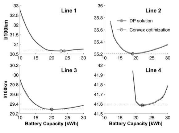
Results from paper:

Source files\tools

References

P. Elbert, T. Nüesch, A. Ritter, N. Murgovski and L. Guzzella, "Engine On/Off Control for the Energy Management of a Serial Hybrid Electric Bus via Convex Optimization," in IEEE Transactions on Vehicular Technology, vol. 63, no. 8, pp. 3549-3559, Oct. 2014.

Published with MATLAB® R2018a