Learning Social Infectivity in Sparse Low-rank Networks Using Multi-dimensional Hawkes Processes
ECE 602 Term Project
Winter 2018
Author: Yanbing Jiang 20501974 & Zirui Wu 20740156
Professor: Oleg Michainovich TA: Mohammad Hossein Basiri
--------------------------------------------------------------------------
Contents
Introduction
In the provided paper, the authors set a goal to solve the problem of inferring the network of social influence from the dynamics of the historical events observed on many individuals, and try to producing a predictive model to answer quantitaively of the following question: when will the indivial inside the society take an action given that some other individuals have already done that.
To address this, the authors proposed a regularized convex optimization approach to discovering the hidden network of social influence based on multi-dimentional Hawkes Process.
From a modeling perspective, the authors would like to take into account several key features of social influence between people and/or among societies/communities (will be discussed later).
Additionally, the multi-dimensional Hawkes process captures the mutually-exciting and recurrent nature of individual behaviours who are active in the social activities, while the regularization using different kind of norms on the infectivity matrix to allow the observer to impose priors on the network topology.
Data Synthesis and Data Generation
- The training data used in this project is systhesised by sampling from a multi-diumensional Hawkes Processes.
- Hawkes Processes is a counting process N(.). An important measure for a counting process is the conditional intensity, as mentioned in the paper. This is defined in the following equation.
![$$\lambda ^{*}=\lim_{h\rightarrow 0} \frac{E[N(t+h)-N(t)|H(t)]}{h}$$](main_eq06784539873702599878.png)
Where H(t) is the historical events. Intuitively, conditional intensity times time interval h is the probability that an event occurs during this infinitesimal interval. Conditional intensity is crucial in sythesizing our training data. However, it is not defined in the original paper.
- The conditional intensity for the u-th dimension in multi-dimensional Hawkes Processes is written below:
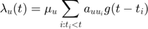
where  is defined as the base intensity for u-th dimension in Hawkes processes.
  corresponds to an element in matrix
  which characterizes the mutual exciting coefficients. is called infectivity matrix.
  is kernel function, which is taken be to be a 1-d Gaussian function as shown in the following:
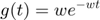
The following function is built for this kernel funciton:
function g = kernel_g(dt, w)
   % Kernel Function defined in the paper
   g = w * exp(-w .* dt);
   % Debugging to set value which has ripple effect
   g(g>1) = 0;
end
- In our synthetic data,
 is taken to be 1. The original paper did not specify the exact value of . Small increase/decrease of the value of does not appear to have an observable impact on the final result. To stay true to the original paper, vector
  and matrix
  are generated via sampling from a uniform distribution. is drawn from interval (0,0.001] with 1000 dimensions. To make sure is both low-rank and sparse, is computed by
  , which are drawn from a interval (0,0.1] forU[100*(i)+1:100*(i+2),i], where i = ,2,3,... 9. All the rest of the elements are set to zeros. In addition, the dimension of is [1000,9] and same for
  .
.  are sampled via the exact same distribution and functions. is then scaled by a scalar to make its largest singular value equal to 0.8 which is suggested by the original paper.
Filling in the Matrix and with the following rules for a random data generation with the method mentioned in the paper: * The initial set for the matrix  and are taken to be zeroes. Also, note that both matrices have the same size of 's. * Note that the purpose of Matrix , , and paramter
  would be described in detail the "Proposed Solution" Section.
clc;            % Initialization
clear;
D = 1000;       % Dimension of HP
U = zeros(D,9); % Initialization of Matrix U
V = zeros(D,9); % Initialization of Matrix V

for i = 1:9
    U(100*(i-1)+1:100*(i+1),i) = rand(200,1)/10;
    V(100*(i-1)+1:100*(i+1),i) = rand(200,1)/10;
end
A = U*V';
A = 0.8 * A./max(abs(eig(A)));
- On the other hand, as illustrated in the paper, is start from a random generated value:
mu = rand(D,1)/D; % True Parameter 1000 dim vector
w = 1;            % w in the kernel function, to be 1 as stated above
- The original paper does not specify which algorithm is used to synthesize training data. Hence, after some reading and experimenting we chose to use the following algorithm called simulation by thinning when synthesising our training data.

- Original paper does not specify number of events to be drawn in each sample. By studying mathematical notation used in the original paper, we presume that that is number is controlled by two variables. Namely the maximum time (Tc) and maximum number of samples (Nc). The event sampling for each one is complete whenever one maximum is reached. However, this approach has two issues. First, the variables are not specified numerically. We assume these two should be in a range so that the number of events (length of each matrix in matlab) across 50,000 samples are more or less the same. This brings out the second issue, matrix size for each sample is different. This means all the samples can not be stacked together without doing padding. Therefore, in our data synthesis only Nc is used as the termination variable and it is taken to be 100.
- Some thoughts are data synthesizing (or in mathematical term, sampling from a distribution).Since this is a multi-dimensional process (with 1000 dimensions),it takes approximately 100 hours to sample all 50,000 data,using a multi-threaded python program without thinning. To significantly reduce the sampling time, thinning is used as illustrated above and the time interval is sampled from distribution as well. The key part is the randomness in the time interval.This assures that different samples have different values even when the time interval is large.
Following is the process of generating the samples of multi-dimention Hawkes Process with the accumulation time utilized for the sample generation:
num_samples = 250; % the number of sequences
nc = 100; % the maximum number of events per sequence
hp_samples = gen_hp_samples(w,mu,A, num_samples,nc); % generating samples
#samples=10/250, time=0.28sec
#samples=20/250, time=0.36sec
#samples=30/250, time=0.42sec
#samples=40/250, time=0.50sec
#samples=50/250, time=0.56sec
#samples=60/250, time=0.62sec
#samples=70/250, time=0.66sec
#samples=80/250, time=0.71sec
#samples=90/250, time=0.77sec
#samples=100/250, time=0.81sec
#samples=110/250, time=0.86sec
#samples=120/250, time=0.91sec
#samples=130/250, time=0.96sec
#samples=140/250, time=1.01sec
#samples=150/250, time=1.06sec
#samples=160/250, time=1.11sec
#samples=170/250, time=1.16sec
#samples=180/250, time=1.21sec
#samples=190/250, time=1.26sec
#samples=200/250, time=1.31sec
#samples=210/250, time=1.35sec
#samples=220/250, time=1.39sec
#samples=230/250, time=1.43sec
#samples=240/250, time=1.48sec
#samples=250/250, time=1.52sec
The sample generated will have a structure as following with events and timestampts:

- The Detail of the function of function hp_samples = gen_hp_samples(w,mu,A, num_samples,nc) will be given in the following:
- The detailed idea of the sample generation could be founded here: https://arxiv.org/pdf/1708.06401.pdf.
function hp_samples = gen_hp_samples(w,mu,A, num_samples,nc)
tic;
hp_samples = struct('timestamp', [],'event', []);
for n = 1:num_samples
    t=0;
    timestamp_and_event = [];
    lambdat = mu;                               % mu is the 1000 dim vector base intensity
    lambdat_sum = sum(lambdat);                 % Sum of all base intensities,used for gen next time-step
    while size(timestamp_and_event, 2) < nc
        rand_u = rand;
        dt = random('exp', 1/lambdat_sum);      % For generating the next time step
        lambda_ts = comp_lambda(t+dt, [], t, lambdat,w,mu,A);
        lambdats_sum = sum(lambda_ts);
        if rand_u > lambdats_sum / lambdat_sum  % Discard sample
            t = t+dt;
            lambdat = lambda_ts;
        else                                    % Keep sample
            u = rand * lambdats_sum;
            lambda_sum = 0;
            for d=1:length(mu)                  % d=1:1000
                lambda_sum = lambda_sum + lambda_ts(d);%sum over all lamda one by one
                if lambda_sum >= u              % Decide which dim event occurs
                    break;                      %end if
                end
            end
            lambdat = comp_lambda(t+dt, d, t, lambdat,w,mu,A);
            t = t+dt;
            timestamp_and_event = [timestamp_and_event,[t;d]];%append new sample
        end
        lambdat_sum = sum(lambdat);            % Time difference for next loop
    end                                        % While size(timestamp_and_event, 2)<nc
    hp_samples(n).timestamp = timestamp_and_event(1,:);
    hp_samples(n).event = timestamp_and_event(2,:);
    if mod(n, 10)==0                           % Print out the generation process
        fprintf('#samples=%d/%d, time=%.2fsec\n',n, num_samples, toc);
    end
end                                            %for n = 1:num_samples
Proposed Solutions
- The objective function and overall minimization algorithm used in the paper is summarised below:

- The objective for optimization is explained as following:
 is the negative log likelihood of the Hawkes Process. The construction of the objective function is based on log-likelyhood function as mentioned in the paper.This is the main and core function that we are trying to make optimization on. and are two variables that we need to obtain from the process of optimization. In addition. and are used in synthesizing the training data as well (which will be covered in the following section soon). Their values are embedded in the training data and we are trying to recover the original value through the process of optimization. On the other hand, and are approximated by iteratively solving the step variables (in terms of step k)
  and
and  . and are Lagrange variables used for the iterative updates. Also, and are chosen from the solution that are given below:

- On the other hand, the and will be both formulated for the property of sparse and lowrank. According to the paper, most individuals only influence a small number of hubs with wide spread influence on many others, which cause the sparsity of the matrix. Furthermore, people tend to form communities, with the likelihood of taking an action increased under the influence of other members of the same community (either assortative or dissortative, and during the experiment, we chose assortative due to computational resources limitations) which leads to sophisticated low-rank structures for the and matrix.
- Following is the main iterative Algorithm (Named ADMM-MM(ADM4)) proposed by the author of the paper:

First of all, there appears to be a TYPO by the authors in the algorithm above (ADM4). The first line immediately after the first while loop should be updating and instead of  and
and  . Futhermore, the first line after the second while loop should be updating and instead of and . After this adjustment, the algoritm then tends to match the content of other parts of the original paper.
Our code is structured after making the adjustment over the algorithm above. An inner function optimization and (the second while loop) and another function on top of that doing the first while loop as well as the initialization of paramaters. One thing worth noting is that only and are returned after the algorithm ends. All the other parameters are either fixed during the procedure of traning samples or training variables assisting the optimization of and .
Furthermore, the convergence condition is not numerically stated by the original paper. Hence in our program, we used both a fixed number of iterations and the threshold condition on the current error to break the while loop, which may be executed a huge number of time.
%start optimization
num_iter_1 = 2;    % Number of Iteration of the First while loop (while k = 1,2 ...)
num_iter_2 = 7;    % Number of Iteration of the Second while loop (while not converge)
rho = 0.09;
thold = 1;         % thershold value
Some Notes:
- Recall the objective function mentioned above (function Q), which is used the second while loop in the ADM4 algorithm. The element that squared in red is what appears to be a typo by the authors. Instead of
 , it should be
  to make sense that the timestamp is focused on a specific sample. Or, this could lead to a ripple effect causing the optimization to fail if we proceeeded with the typo.
 - Furthermore, the element that squared in green is another typo we found in the objective function. As the term
 has never been mentioned in the paper from the beginning the end, we guessed that it should be replaced by
  , which has been formulated in the log-likelihood function in the paper, and make sense for the term to be specified upon a sample
  .
. - There are lots of sums between two variables as well. These variables could be added one by one or parallelized through vector and/or matrix calculation. For instance, whle calculating the value of
 and , they could be treated as a vector. Thus, the summation is simply an inner product between those two variables. This parallelization idea is implemented in several parts of our code while doing the optimization.
Implementation of the Solutions
- With the Objective function and algorithm listed, we have built a function that is utilize to make optimization over and iteratively.
- The output of the function
 is the optimized result of , while
  is the corresponding optimized result of . Furthermore, the output Iteration_Err is in the function is the a list error during each iteration.
[x,y,Iteration_Err] = optimize_a_mu(hp_samples,D,w,rho,num_iter_1,num_iter_2,thold,A);
No. 1 outter while iteration | No. 1 inner while iterationnon-zero in mu= 1000
non-zero in C= 604531
non-zero in B = 1000000, non-zero in sqrt = 1000000
real error = 0.9609, correlation = 0.1688, #non-zero in A = 532775

No. 1 outter while iteration | No. 2 inner while iterationnon-zero in mu= 1000
non-zero in C= 532775
non-zero in B = 532775, non-zero in sqrt = 532775
real error = 0.4003, correlation = 0.0645, #non-zero in A = 413334

No. 1 outter while iteration | No. 3 inner while iterationnon-zero in mu= 1000
non-zero in C= 413334
non-zero in B = 413334, non-zero in sqrt = 413334
real error = 0.2981, correlation = 0.0133, #non-zero in A = 330105

No. 1 outter while iteration | No. 4 inner while iterationnon-zero in mu= 1000
non-zero in C= 330105
non-zero in B = 330105, non-zero in sqrt = 330105
real error = 0.2869, correlation = 0.0030, #non-zero in A = 267133

No. 1 outter while iteration | No. 5 inner while iterationnon-zero in mu= 1000
non-zero in C= 267133
non-zero in B = 267133, non-zero in sqrt = 267133
real error = 0.2849, correlation = 0.0010, #non-zero in A = 216017

No. 1 outter while iteration | No. 6 inner while iterationnon-zero in mu= 1000
non-zero in C= 216017
non-zero in B = 216017, non-zero in sqrt = 216017
real error = 0.2841, correlation = 0.0005, #non-zero in A = 172956

No. 1 outter while iteration | No. 7 inner while iterationnon-zero in mu= 1000
non-zero in C= 172956
non-zero in B = 172956, non-zero in sqrt = 172956
real error = 0.2837, correlation = 0.0003, #non-zero in A = 135350

No. 1 outter while iteration | No. 8 inner while iterationnon-zero in mu= 1000
non-zero in C= 135350
non-zero in B = 135350, non-zero in sqrt = 135350
real error = 0.2834, correlation = 0.0002, #non-zero in A = 101753

No. 2 outter while iteration | No. 1 inner while iterationnon-zero in mu= 1000
non-zero in C= 101753
non-zero in B = 101753, non-zero in sqrt = 101753
real error = 0.2831, correlation = 0.0002, #non-zero in A = 73060

No. 2 outter while iteration | No. 2 inner while iterationnon-zero in mu= 1000
non-zero in C= 73060
non-zero in B = 101753, non-zero in sqrt = 101753
real error = 0.2829, correlation = 0.0001, #non-zero in A = 49428

No. 2 outter while iteration | No. 3 inner while iterationnon-zero in mu= 1000
non-zero in C= 49428
non-zero in B = 101753, non-zero in sqrt = 101753
real error = 0.2828, correlation = 0.0001, #non-zero in A = 32331

No. 2 outter while iteration | No. 4 inner while iterationnon-zero in mu= 1000
non-zero in C= 32331
non-zero in B = 101753, non-zero in sqrt = 101753
real error = 0.2827, correlation = 0.0000, #non-zero in A = 21096

No. 2 outter while iteration | No. 5 inner while iterationnon-zero in mu= 1000
non-zero in C= 21096
non-zero in B = 101753, non-zero in sqrt = 101753
real error = 0.2826, correlation = 0.0000, #non-zero in A = 14011

No. 2 outter while iteration | No. 6 inner while iterationnon-zero in mu= 1000
non-zero in C= 14011
non-zero in B = 101753, non-zero in sqrt = 101753
real error = 0.2826, correlation = 0.0000, #non-zero in A = 9622

No. 2 outter while iteration | No. 7 inner while iterationnon-zero in mu= 1000
non-zero in C= 9622
non-zero in B = 101753, non-zero in sqrt = 101753
real error = 0.2825, correlation = 0.0000, #non-zero in A = 6785

No. 2 outter while iteration | No. 8 inner while iterationnon-zero in mu= 1000
non-zero in C= 6785
non-zero in B = 101753, non-zero in sqrt = 101753
real error = 0.2825, correlation = 0.0000, #non-zero in A = 4972

No. 3 outter while iteration | No. 1 inner while iterationnon-zero in mu= 1000
non-zero in C= 4972
non-zero in B = 101753, non-zero in sqrt = 101753
real error = 0.2824, correlation = 0.0000, #non-zero in A = 3777

No. 3 outter while iteration | No. 2 inner while iterationnon-zero in mu= 1000
non-zero in C= 3777
non-zero in B = 101753, non-zero in sqrt = 101753
real error = 0.2824, correlation = 0.0000, #non-zero in A = 2870

No. 3 outter while iteration | No. 3 inner while iterationnon-zero in mu= 1000
non-zero in C= 2870
non-zero in B = 101753, non-zero in sqrt = 101753
real error = 0.2823, correlation = 0.0000, #non-zero in A = 2261

No. 3 outter while iteration | No. 4 inner while iterationnon-zero in mu= 1000
non-zero in C= 2261
non-zero in B = 101753, non-zero in sqrt = 101753
real error = 0.2823, correlation = 0.0000, #non-zero in A = 1796

No. 3 outter while iteration | No. 5 inner while iterationnon-zero in mu= 1000
non-zero in C= 1796
non-zero in B = 101753, non-zero in sqrt = 101753
real error = 0.2823, correlation = 0.0000, #non-zero in A = 1480

No. 3 outter while iteration | No. 6 inner while iterationnon-zero in mu= 1000
non-zero in C= 1480
non-zero in B = 101753, non-zero in sqrt = 101753
real error = 0.2823, correlation = 0.0000, #non-zero in A = 1236

No. 3 outter while iteration | No. 7 inner while iterationnon-zero in mu= 1000
non-zero in C= 1236
non-zero in B = 101753, non-zero in sqrt = 101753
real error = 0.2823, correlation = 0.0000, #non-zero in A = 1069

No. 3 outter while iteration | No. 8 inner while iterationnon-zero in mu= 1000
non-zero in C= 1069
non-zero in B = 101753, non-zero in sqrt = 101753
real error = 0.2823, correlation = 0.0001, #non-zero in A = 943
- Following show the detail of the optimize_a_mu function:
function [A_m,mu_m,Iteration_Err] = optimize_a_mu(hp_samples,D,w,rho,num_iter_1,num_iter_2,thold,real_A)
    % Input the training samples, parameters, number of iterations
    % and the real A for iterative learning.
    A_m = rand(D,D);          % Start with a random matrix to make optimization
    A_m = 0.8 * A_m./max(abs(eig(A_m)));  % Similar with the real A, scale the spectral radius of A_m to 0.8
    mu_m = rand(D, 1)./D;     % Start with a random mu value to make optimization as well
    UL = zeros(D,D);          % Matrix U's Parameter of Lowrank Property
    ZL = zeros(D,D);          % Matrix Z's Parameter of Lowrank Property
    US = zeros(D,D);          % Matrix U's Parameter of Sparse Property
    ZS = zeros(D,D);          % Matrix U's Parameter of Sparse Property
    %
    for i = 0:num_iter_1      % Outer while loop for algorithm 1 in the paper
		    rho = rho * 1.1;      % Iteratively change the value of rho each time
        for j = 0:num_iter_2  % Inner while loop for algorithm 1 in the paper
            % Main Algorithm mentioned above
            fprintf('No. %d outter while iteration | No. %d inner while iteration', i+1,j+1);
			    [A_m,mu_m,RelErr] = update_a_mu(A_m,mu_m,hp_samples,UL,ZL,US,ZS,w,rho,D,real_A);
            Iteration_Err(j+1,i+1) = RelErr;   % Capture the error during each iteration
        end
		    [s,v,d] = svd(A_m + US);     % Update ZL via SVD (Singular Value Decomposition)
		    v = v - thold/rho;
		    v(v < 0) = 0;                % Get ride of negatives
		    ZL = s * v * d';             % Update ZL (Z for LowRank)
		    UL = UL + (A_m - ZL);        % Update UL (U for LowRank)
		    tmp = (abs(A_m + US)-thold/rho);
		    tmp(tmp < 0) = 0;
		    ZS = (sign(A_m + US).*tmp);  % Update ZS (Z for Sparse)
		    US = US + (A_m-ZS);          % Update US (U for Sparse)
    end
 end
The above function is the frame of optimization to update and , which includes iteration frame and the updates over matrix and under the condition of Lowrank and Sparse respectively. The core update function that used to update parameter is called update_a_mu(.), which is a demonstration of the algorithm ADM4 stated above. the function code is shown as following:
function [A,mu,RelErr] = update_a_mu(A_m,mu_m,hp_samples,UL,ZL,US,ZS,w,rho,D,real_A)
    num_samples = length(hp_samples);
    %following the Algorthm 1: ADM4
    mu_numerator = zeros(D, 1);%init [D,1] all zeros; D -> dim of HP
    C = zeros(size(A_m));           % Initiation of the Matrix C (Equation 10 in the paper)
    A_Step = zeros(size(A_m)) + 2 * rho;
    B = zeros(size(A_m)) + rho*(UL-ZL) + rho*(US-ZS);% Add rho to B and its initialization (Equation 10 in the paper)
    for s = 1:num_samples           % Iterate through all the samples, 50,000
        timestamp = hp_samples(s).timestamp;% A vector, let's say 100 time stamps
        event = hp_samples(s).event;% A vector, each value a dim, same size as Time
        tc = timestamp(end);        % End time
        nc = length(event);
        dt = tc - timestamp;        % dt for all every time step
        for i = 1:nc                % Iterate through all the timestamps and events in ONE sample
            ui = event(i);          % Scalar
            ti = timestamp(i);      % Scalar
            int_g = kernel_int_g(dt, w);
            B(ui,:) = B(ui,:) + double(A_m(ui,:)>0).*repmat(int_g(i),[1,D]);
            pii = [];               % Initiation of the pii parameter is the Q objective function (Equation 8 in the paper)
            pij = [];               % Initiation of the pij parameter is the Q objective function (Equation 8 in the paper)
            ag_arr = [];            % Sum Auiuj*g(ti-tj)
            if i>1
                tj = timestamp(1:i-1);                        % Vector
                uj = event(1:i-1);                            % Vector
                ag_arr = A_m(uj, ui) .* kernel_g(ti - tj, w)';% Vector
            end
            pii = mu_m(ui)./(mu_m(ui) + sum(ag_arr));    % Calculation of pii in Equation 8 in the paper
            if i>1
                pij = ag_arr./(mu_m(ui) + sum(ag_arr));  % Calculation of pij in Equation 8 in the paper
                if ~isempty(pij) && sum(pij(:))>0
                    for j = 1:length(uj)
                        uuj = uj(j);
                        C(uuj,ui) = C(uuj,ui) - pij(j,:);% Calculation of matrix C in Equation 10 in the paper
                    end
                end
            end
            mu_numerator(ui) = mu_numerator(ui) + pii;
        end                                           % for i = 1:nc (number of sequence in a sample)
    end                                               % for s = 1:num_samples (number of samples)
    mu = mu_numerator./(zeros(D, 1) + tc);            % Equation 9 in the paper
    A = (-B + sqrt(B.^2 - 4*A_Step.*C))./(2*A_Step);  % Equation 10 in the paper % Given AmatA = zeros(size(A_m)) + 2 * rho;
    RelErr = real_err(real_A,A);                      % Storage of Iteration Relative Error
    fprintf('non-zero in mu= %d\n',nnz(mu));          % Testing of the sparse consition for mu
    fprintf('non-zero in C= %d\n',nnz(C));            % Testing of the sparse consition for C
    fprintf('non-zero in B = %d, non-zero in sqrt = %d\n',nnz(B),nnz(sqrt(B.^2 - 4*A_Step.*C)));
    fprintf('real error = %.4f, correlation = %.4f, #non-zero in A = %d\n\n',real_err(real_A,A),sum(abs(corr(real_A(:),A(:)))),nnz(A));
    A(isnan(A))=0;                                    % Refer to Equation 10 in the paper
    A(isinf(A))=0;
    %(A==0) = 0.00001;
  end                                                 %end function
- Note that the real_err is the relative error that we need to collect during the iteration of the computation, the function of real_err(.) is listed as following:
function err = real_err(A,A_m)
   % The calculation od relative error
   % Relative error is defined as the averaged
   % relative error between the estimated parameters
   % and the true parameters
   % i.e aij != 0 then err = err_1 or err = err_2 defined following.
    err_1 = abs(A - A_m) ./ A;
	    err_2 = abs(A - A_m);
	    err_1(isnan(err_1))=0;
    err_1(isinf(err_1))=0;
	    err = err_1 .* double(A~=0) + err_2.*double(A==0);
	    err = sum(err(:))/double(numel(A));
end
Debugging and Improvements
- Handling of Nan (not a number) and Inf (infinity): Nan and Inf has a 'ripple effect'. Namely, if they are not dealt with properly, our would , after certain number of iterations become all Infs and Nans. For example, Infs could be caused by dividing by 0. is assumed to be sparse, therefore this is common situation that could happen. To fix this, we can divide only by non-zero numbers or set 0 to a very small number. Just to ensure the stability of our programming, we set all Infs and Nans in Matrix to zeros at the end of each iteration as a solution (as shown in the last third and fourth line of the code above.
- Synatic/Logical Errors vs. Numerical Errors: The normal approach is to check logical errors in the program firstly before checking the value of hyper-parameters. However, in this case, checking logical errors could be very tedious since there are too many summation signs. As the dimension of samples from the Hawkes Process is huge (i.e. 1000), there is no good way to systematically figure out which error it is during debugging, and lots of time were spent on this.
- Handling Break Conditions: The original paper does not specify a convergence condition during the operation of the algorithm. The computation cost in each iteration is the same. However, improvements decrease gradually because of this. Instead of proposing a numerical value for convergencem, we chose to fix the number of iterations of each loop (as indicated above in the section of 'Proposed Solution'). This has an extra benefit that the program will not stuck in an infinite loop if it does not converge to the threshold value that we set.
Learning Results
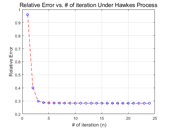
As the result as permutated according to the number of iterations in outter and inner while loop, we, firstly, repermutated the errors into a vector and then plot the corresponding relative error vs number of iteration plot with the following codes.
Iteration_Err2 = reshape(Iteration_Err,[],1);
figure('Name','Relative Error vs. # of iteration Under Hawkes Process');
plot(Iteration_Err2,'--ro','LineWidth',1,'MarkerSize',5,'MarkerEdgeColor','b');
grid;
title('Relative Error vs. # of iteration Under Hawkes Process', 'FontSize',14);
set(gca,'YTick',0:0.1:2.2);
xlabel(' # of iteration (n)','FontSize',12);
ylabel('Relative Error','FontSize',12);
Conclusions and Thoughts
- As shown in the plot, our experiment tends to converge to an error (this is the RelErr on pg.645 in the paper) rate of approximately 0.28 instead of the nearly 0.2 error in the original paper. This, by oyr estimation is partially result of lack of specific hyper-parameters. Although the value for the matrix and vector are specified, some of the parameters like
 and the amount of increments after each iteration are not numberically specified. These hyper-parameters are crucial in terms of reproducing a close error rate. By setting 10 times larger (e.g. 0.09 to 0.9) could lead to disastrous results. Erro rate increases instead of dropping after each iteration and we had to debug the program that is structurally correct.
- Although our work suggests that the optimization algorithm proposed by the original paper is correct and seems to work by our experiments utilizing MATLAB, the paper itself is not friendly in helping us reproducing its work. Lack of specific efficient sampling algorithm and explanation of what conditional intensity is forced us to spend lots of efforts on figuring out how to sample from a multi-dimensional Hawkes Process. We have found at least 3 critical typos in the original papers as well (mentioned above). Typos caused us some confusion while trying to comprehend the paper to do the job of reproducing. Also, the typos in equations if implemented exactly would produce error and would never approach the desired results.
- Abuse of Math Notation:

This triple summation in Equation 10 in the original paper (element Matrix C) used three different conventions: the subscrpts for the last two summation signs are squeezed together and we have to infer from the words on how it is contrcuted. Using and together, although technically correct, did make it hard for the readers to figure out what each variable is. Also convention states capital letters should be used for matrix only instead of an element in the matrix.
- Result Explanations: due to the time limitation and the computational resource limitation. We finally take the experiment with the sample size of 250 instead all 10000,20000,30000,40000 and 50000 samples.Normally, but separate observation, the trend of error would look like as following:

Reference List
- [1] Learning Social Infectivity in Sparse Low-rank Networks Using Multi-dimensional Hawkes Processes . K.Zhou, H. Zha, L. Song, 2013. [Online]. Available: http://proceedings.mlr.press/v31/zhou13a.pdf, Accessed: Apr.5, 2018.
- [2] A Tutorial on Hawkes Processes for Events in Social Media . M. Rizoiu, Y.Lee and etc. [Online]. Available: https://arxiv.org/pdf/1708.06401.pdf, Accessed Apr.10, 2018.
Source files and functions
- Multi-dimension Hawkes Process Simulation:
comp_lambda.m: function for computing lambda in the paper iteratively.
gen_hp_samples.m: function for generating samples.
- Optimization:
update_a_mu.m: function for computering the inner loop. Solve A,mu via equation 10.
optimize_a_mu.m: function for solving and via all the samples.
- Validation:
real_err.m: function for checking error between and 
- Utility functions (for kernel functions):
kernel_g.m: function for calculating exp kernel
kernel_G.m: function for calculating integration of the exp kernel