GA-based method for feature selection and parameters optimization for machine learning regression applied to software effort estimation
Department of Electrical and Computer Engineering - University of Waterloo, Waterloo, ON, Canada
Introduction to optimization (ECE 602) - Instructor: Prof. Oleg Michailovich
course project - Winter 2018
Team members:
- Hadi Nekoeiqachkanloo (Waterloo ID: 20727088)
- Benyamin Ghojogh (Waterloo ID: 20743301)
Contents
- 1) ======= Problem Description and Formulation
- 1-1) Introduction to problem
- 1-2) Feature selection
- 1-3) Parameters of SVR
- 1-4) Parameters of MLP neural network
- 1-5) Parameters of M5P
- 1-6) Summarizing the parameters of regressors
- 2) ======= Proposed Optimization Solution
- 2-1) Short description of Genetic Algorithm (GA)
- 2-2) Modeling chromosomes for effort estimation problem
- 2-3) Fitness for effort estimation problem
- 2-4) Two-point crossover
- 2-5) Roulette Wheel selecition
- 2-6) Elitism replacement
- 2-7) Flow chart of the proposed algorithm
- 2-8) Settings of the utilized GA algorithm
- ======= 3) Data Sources
- 3-1) Datasets and their details
- 3-2) Train/Test splits in the datasets
- 3-3) MATLAB initializations and some settings
- 3-4) Reading datasets and fixing missing values
- 3-5) Preprocessing COCOMO dataset
- 3-6) Dividing the COCOMO dataset into six train/test datasets
- 4) ======= Solution
- 4-1) Overall k-fold cross validations and running GA
- 4-2) The binary_GA function
- 4-3) The calculate_fitness function
- 4-4) The report_experimental_results function
- 5) ======= Results
- 5-1) Metrics of the evaluations used in paper [1]
- 5-2) Results of Desharnais dataset
- 5-3) Results of NASA dataset
- 5-4) Results of COCOMO dataset
- 5-5) Results of Albrecht dataset
- 5-6) Results of Kemerer dataset
- 6) ======= Analysis and Conclusions
- 6-1) Time complexity and settings of the proposed algorithm
- 6-2) Our critiques on the paper [1]
- 6-3) Analysis and comparison of the results
- 7) ======= List of Used Files
- 8) ======= References
1) ======= Problem Description and Formulation
1-1) Introduction to problem
In this report, we recreate and comment on the results of the paper "GA-based method for feature selection and parameters optimization for machine learning regression applied to software effort estimation" [1].
The paper [1], which is implemented and reproduced in this project, deals with the application of software effort estimation. Software effort estimation tries to estimate the human-hour effort required for producing a special software regarding the characteristics of it. One of the ways for estimating the effort is regression in machine learning. There are different regression methods existing in machine learning which are widely used for software effort estimation, such as:
- Radial Basis Function (RBF) neural network
- Multi-layer perceptron (MLP) neural network
- regression trees
- wavelet neural network
- bagging predictors
- Support Vector Regression (SVR)
The paper [1] uses four regression methods, which are:
- SVR (with RBF kernel)
- SVR (with linear function)
- MLP neural network
- M5P tree (a type of regression tree)
The two main goals of paper [1] are:
- Optimizing the parameters of the regression methods
- Finding the most discriminating features (feature selection)
This paper utilizes binary Genetic Algorithm (GA) for doing the two above goals (which will be explained in the next section).
In the following, the feature selection is explained:
1-2) Feature selection
In regression problem, the features of i-th sample can be denoted as a column vector  . The observation (or output) of this feature is denoted by a scalar
  . Here, observations are efforts of software development. All the features can be put together row-wise in a matrix denoted by
 ![$X = [x_1^T; \dots, x_n^T]$](main_eq03150331592919124928.png) and its labels
and its labels ![$Y = [y_1, \dots, y_n]^T$](main_eq03568948977243318800.png) . Feature selection means that we select the specific columns of matrix
. Feature selection means that we select the specific columns of matrix  which help the description in regression the best.
1-3) Parameters of SVR
In Support Vector Regression, we try to maximize the distance of boundary from the samples of different labels. This is equivalent to minimizing the absolute value of normal vector  of the boundary hyperplanes. So, the optimization problem of SVR is formulated as [1]:
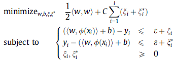
where parameters  and
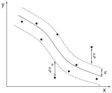
and  are called slack variables and measure the cost of the errors on the training points. The measures deviations exceeding the target value by more than
  and measures deviations which are more than below the target value. This can be seen in the following figure [1,5]:
The parameter  is the complexity of SVR model. The larger this parameter gets, the more the slack variables are penalized in the optimization problem, so the boundary gets more restricted to separate the different labels more correctly.
The kernel trick is that we project the data to a higher dimensional hyperspace so that data become more discriminated in that higher dimensional space. The Radial Basis Function (RBF) kernel is  where and
  respectively denote the training and testing data sample. The larger the parameter
  gets, the more bias (less variance) the model will have so that its tolerance to deviation from the training pattern gets less. On the other hand, if linear (no kernel trick), the linear kernel is
  .
.
1-4) Parameters of MLP neural network
Multi-layer perceptron is a neural network probably having a hidden layer (there is a universal principal indicating that using a neural nework having merely one hidden layer suffices for classifying/regressing any pattern). In this work, output is a scalar so that we have one output neuron. A sketch of MLP is in the following figure [2]:
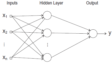
The MLP regressor has the parameters of number of nodes in hidden layer  , number of training epochs (iterations)
  , learning rate in the backpropagation algorithm
  , and the momentum rate foe the backpropagation algorithm
  .
.
1-5) Parameters of M5P
M5P is a model tree which is used in this work. Model trees are special types of decision trees used for regression. The smoothing can be done for compensating the discontinuities of the regression in the tree. So, smoothing or not smoothing is a parameter. Another parameter is whether pruning or not pruning the tree after growing it. Another parameter is minimum number of samples in every leaf of tree. This parameter controls how deep the tree can grow.
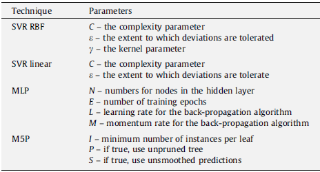
1-6) Summarizing the parameters of regressors
The mentioned parameters in the utilized regression methods can be summarized in the following table [1]:
2) ======= Proposed Optimization Solution
The paper [1] tries to optimize the selected features and the parameters of regressors using Genetic Algorithm (GA) with binary chromosomes.
2-1) Short description of Genetic Algorithm (GA)
Genetic algorithm is a metaheuristic optimization algorithm which tries to find the global minimum of a cost function using several particles which are chromosomes in this algorithm. There are several chromosomes which try to find the global optimum together. The idea of genetic algorithm is based on evolution and Darwinism. Initially, the chromosomes are distributed in the search space (landscape of cost function). Note that every chromosome is a possible solution to the optimization problem. The cost of cost function for each chromosome is calculated and then they are sorted based on their cost in ascending order. The chromosomes with less cost are better chromosomes in terms of evolution and their features should transfer to the next generaion with a higher chance. So, the chromosomes are selected pairwise randomly with the probabilities proportional to their cost (the less cost they have, the more chance of selection they have). Then, the result of mating of pairs of chromosomes is two chromosome children having properties of their parents in part. This step of algorithm is named "crossover". This crossover handles the "exploitation" which means that the algorithm tries to search around the best solutions found so far. Afterwards, in order to avoid getting stuck in local minimum, we apply some "mutations" in the child chromosome, meaning that we change its bits from 0 to 1 or vice versa. This garantees exploration which means that the algorithm tries to explore and search other locations in the search space for a possible better solution.
2-2) Modeling chromosomes for effort estimation problem
The chromosome is divided into two parts, (I) genes for parameters, and (II) genes for feature selection. Each parameter is associated  bits (genes) in binary representation. Paper [1] sets
  . In order to convert the binary representation of each parameter (genotype) to the decimal value of parameter (phenotype) in its range [min(p), max(p)], we can use the following equation:
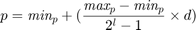
where  is the decimal value of the binary representation of the parameter in the chromosome. Note that the paper [1] does not report the
  and
and  in their paper and say that these values cam be decided by user.
For the feature selection part, on the other hand, every bit (gene) determines whether the feature is selected (bit 1) or not selected (bit 0). The structure of the chromosome is showin in the following figure:

2-3) Fitness for effort estimation problem
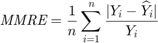
In metaheuristic optimization algorithms, if the problem is minimization, cost function is usually used and fitness function is mostly utilized for maximization. However, the paper [1] uses fitness function terminology as cost function. The fitness of optimization problem consists of two metrics. The first metric is MMRE which is:
The second metric is PRED(25) which is the percentage of predictions that fall within  of the actual value. This metric is formulated as [2]:

where  is the total number of samples and
  is the number of samples whose
  values are less than or equa to 0.25.
The fitness function is then defined as [1]:

However, paper [1] uses merely 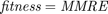 for COCOMO dataset, inspired by paper [10].
2-4) Two-point crossover
Paper [1] uses the two-point crossover. In this type of crossover, two points are randomly selected in the two parents whose locations are similar on the two parents. So, every parent is divided into three parts. The first and last parts of a parent and the middle part of the other parent makes the new child. The other child is made by the opposite parts of the parents. This process is illustrated in the following figure:

2-5) Roulette Wheel selecition
Paper [1] uses Roulette Wheel selecition for selecting the parents for crossover abd mating. In Roulette Wheel selecition, a virtual roulette wheel exists in which the less the cost of a chromosome, the larger space (probability) that chromosome has in that roulette wheel. So, the better chromosomes have more chance to be selected. The following figure from [3] shows this (in this figure, larger fitness is better):

2-6) Elitism replacement
Paper [1] uses elitism replacement, which means that for generating next generation, a portion of the best chromosomes are transfered directly to the next generation and the rest population of the next generation are obtained by the crossover of the parents. Note that paper [1] does not mention what portion they use for elitism replacement.
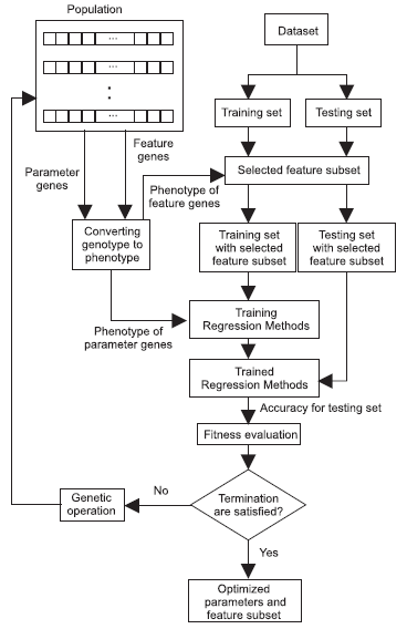
2-7) Flow chart of the proposed algorithm
In the following figure, the flow chart of the prposed algorithm in [1] is depicted. As can be seen in this figure, the dataset is divided into training and testing sets. Initially, the chromosomes are spread in the search space and thus the parameters and the selected features are determined. The features are selected and the parameters are set based on the chromosomes. Then, the regression method is trained for each chromosome and the test set is tested for that chromosome. The fitness of each chromosome is calculated and checked whether the termination criterion has reached or not. The termination check in this paper [1] is reaching the maximum number of generations. IF termination is not reached, the next generation of GA is generated and the selected features and the parameters are determined again and the previously explained steps are repeated.
2-8) Settings of the utilized GA algorithm
The paper [1] has tested these settings for the settings of GA algorithm: (I) population size = {50, 100, 200, 300, 500}, (II) number of generations = {20, 25, 50, 100, 200}, (III) crossover rate = {0.5, 0.6, 0.65, 0.7, 0.8}, and (IV) mutation rate = {0.05, 0.1, 0.2, 0.3}. Finally, the paper [1] says that they have selected the parameters as (I) population size = 500, (II) number of generations = 25, crossover rate = 0.8, mutation rate = 0.3, and all the results of experimental results in [1] are using these settings. Moreover, paper [1] runs the GA algorithm for 10 times (because of randomness of the GA algorithm) and take the average of these results.
Notice that for each chromosome, we should train and test once, and there are 500 chromosomes in every generation, and there are 25 generations, and there are several folds in the cross validation. Moreover, they do run the proposed algorithm for 10 times. Thus, as we discuss later in section 6, the experthe program takes a long time (probably weeks) to run. So, we relax these settings because of lack of time. Because it is impossible to run all the program before the deadline. The taken setup in this project will be reported in the section 6 (please see that section for seeing the taken settings in this project).
======= 3) Data Sources
3-1) Datasets and their details
The datasets used in paper [1] are listed below:
- Desharnais dataset [4]: includes 81 software projects (samples) and 11 features (including index of sample) and 1 output feature (effort). Paper [1] ignores the feature length (fifth feature).
- NASA dataset [5]: includes 18 software projects (samples) and 2 features and 1 output feature (effort).
- COCOMO dataset [6]: includes 63 software projects (samples) and 16 features and 1 output feature (effort).
- Albrecht dataset [7]: includes 24 software projects (samples) and 7 features and 1 output feature (effort).
- Kemerer dataset [8]: includes 15 software projects (samples) and 7 features (including index of sample) and 1 output feature (effort).
- Korten and Gray dataset [9]: includes 17 software projects (samples) and 5 features and 1 output feature (effort).
3-2) Train/Test splits in the datasets
Paper [1] has the following settings for splitting the datasets to training and testing sets:
- Desharnais dataset [4]: randomly selecting 18 samples out of 81 samples for test set. The remaining 63 samples are training samples. To the best of our understanding, paper [1] does not do this split for several times to take average afterwards! Probably the reason is that they run GA algorithm for 10 times.
- NASA dataset [5]: Leave-one-sample-out cross validation (LOOCV) for splitting into train/test sets
- COCOMO dataset [6]: Paper [1] divides COCOMO dataset into training and testing samples in 6 different ways, inspired by paper [10]. The following table shows these 6 different datasets [1].
- Albrecht dataset [7]: Leave-one-sample-out cross validation (LOOCV) for splitting into train/test sets
- Kemerer dataset [8]: Leave-one-sample-out cross validation (LOOCV) for splitting into train/test sets
- Korten and Gray dataset [9]: Leave-one-sample-out cross validation (LOOCV) for splitting into train/test sets

All the mentioned datasets are publicly avaliable in the internet except the Korten and Gray dataset [9] which we could not find it after a lot of search. Thus, we do the experiments on the other five datasets.
3-3) MATLAB initializations and some settings
In the following code, we add the paths of functions and also set the settings which were explained in the above sections.
%%%%%% MATLAB initializations and some parameters and variables:
clc
clear
clear all
close all
addpath('./Functions/')
addpath('./Functions/tree_regression_functions/')
warning('off', 'all')
global report_progress_1; report_progress_1 = 1;  % report dataset
global report_progress_2; report_progress_2 = 1;  % report index of fold
global report_progress_3; report_progress_3 = 1;  % report regression method
global report_progress_4; report_progress_4 = 1;  % report index of simulation
global report_progress_5; report_progress_5 = 1;  % report index of generation in GA
global report_progress_6; report_progress_6 = 0;  % report index of chromosome in GA
global MMRE_overall;
global PRED_25_overall;
global Sum_Ab_Res_overall;
global Med_Ab_Res_overall;
global SD_Ab_Res_overall;
global number_of_removed_features_overall;
population_size = 500;
number_of_generations = 25;
elitism_population = 30;  % notice: (population_size - elitism_population) should be even
crossover_rate = 0.8;
mutation_rate = 0.3;
number_of_GA_simulations = 10;
3-4) Reading datasets and fixing missing values
In the following code, we do the following things:
- Read the datasets from the files
- Fixing the missing (invalid) data: some of the values in the datasets are written as ? which means they are missing. We replace them using the average of that feature.
- Preparing X and Y of datasets. We exclude the indices of samples. We also take efforts as Y according to aim of paper [1]. In dataset Desharnais, feature length is ignored as in [1].
%%%%%% Reading datasets:
number_of_datasets = 5;
data = cell(number_of_datasets, 1);
for dataset_index = 1:number_of_datasets
    if dataset_index == 1
        filename = './Datasets/Desharnais.txt';
        number_of_features = 12;
    elseif dataset_index == 2
        filename = './Datasets/NASA.txt';
        number_of_features = 4;
    elseif dataset_index == 3
        filename = './Datasets/COCOMO.txt';
        number_of_features = 17;
    elseif dataset_index == 4
        filename = './Datasets/Albrecht.txt';
        number_of_features = 8;
    elseif dataset_index == 5
        filename = './Datasets/Kemerer.txt';
        number_of_features = 8;
    end
    fileID = fopen(filename);
    format = '%f';
    for feature_index = 1:number_of_features-1
        format = [format, ' %f'];
    end
    C = textscan(fileID,format,'Delimiter',',',...
        'TreatAsEmpty',{'?'},'EmptyValue',nan);
    fclose(fileID);

    %%%%%% fixing missing data:
    for feature_index = 1:length(C)
        for sample_index = 1:length(C{feature_index})
            if isnan(C{feature_index}(sample_index))
                average_of_feature = nanmean(C{feature_index}); % taking mean ignoring nan values
                C{feature_index}(sample_index) = average_of_feature;
            end
        end
    end

    %%%%%% preparing X and Y of datasets:
    if dataset_index == 1   %--> Desharnais dataset
        data{dataset_index}.features = [];
        for feature_index = 1:length(C)
            if feature_index ~= 1 && feature_index ~= 5 && feature_index ~= 6
                %%%%%% feature_index == 1 --> project ID
                %%%%%% feature_index == 5 --> project length
                %%%%%% feature_index == 6 --> effort
                data{dataset_index}.features = [data{dataset_index}.features, C{feature_index}];
            end
        end
        data{dataset_index}.efforts = C{6};
    elseif dataset_index == 2   %--> NASA dataset
        data{dataset_index}.features = [];
        for feature_index = 1:length(C)
            if feature_index ~= 1 && feature_index ~= 4
                %%%%%% feature_index == 1 --> project ID
                %%%%%% feature_index == 4 --> effort
                data{dataset_index}.features = [data{dataset_index}.features, C{feature_index}];
            end
        end
        data{dataset_index}.efforts = C{4};
    elseif dataset_index == 3   %--> COCOMO dataset
        data{dataset_index}.features = [];
        for feature_index = 1:length(C)
            if feature_index ~= 17
                %%%%%% feature_index == 17 --> effort
                data{dataset_index}.features = [data{dataset_index}.features, C{feature_index}];
            end
        end
        data{dataset_index}.efforts = C{17};
    elseif dataset_index == 4   %--> Albrecht dataset
        data{dataset_index}.features = [];
        for feature_index = 1:length(C)
            if feature_index ~= 5 && feature_index ~= 8
                %%%%%% feature_index == 5 --> FPAdj --> papers don't mention it
                %%%%%% feature_index == 8 --> effort
                data{dataset_index}.features = [data{dataset_index}.features, C{feature_index}];
            end
        end
        data{dataset_index}.efforts = C{8};
    elseif dataset_index == 5   %--> Kemerer dataset
        data{dataset_index}.features = [];
        for feature_index = 1:length(C)
            if feature_index ~= 1 && feature_index ~= 8
                %%%%%% feature_index == 1 --> project ID
                %%%%%% feature_index == 8 --> effort
                data{dataset_index}.features = [data{dataset_index}.features, C{feature_index}];
            end
        end
        data{dataset_index}.efforts = C{8};
    end

end
3-5) Preprocessing COCOMO dataset
Inspired by paper [10], paper [1] preprocesses COCOMO dataset so that the discrmination of features becomes easier. The preprocessing, replaces the values of each feature with a specific value level. The value levels are mostly 1, 2, 3, 4, 5, or 6. The replacements are all mentioned in [10] for all the features of COCOMO dataset.
%%%%%% Preprocessing COCOMO dataset:
X = data{3}.features;
number_of_samples = size(X, 1);
number_of_features = size(X, 2);
for feature_index = 1:number_of_features
    for sample_index = 1:number_of_samples
        value = X(sample_index, feature_index);
        if feature_index == 1  %--> feature: rely
            if value == 0.75  %--> very low
                X(sample_index, feature_index) = 1;
            elseif value == 0.88 || value == 0.94  %--> low
                X(sample_index, feature_index) = 2;
            elseif value == 1  %--> nominal
                X(sample_index, feature_index) = 3;
            elseif value == 1.15  %--> high
                X(sample_index, feature_index) = 4;
            elseif value == 1.4  %--> very high
                X(sample_index, feature_index) = 5;
            end
        elseif feature_index == 2  %--> feature: data
            if value == 0.94  %--> low
                X(sample_index, feature_index) = 1;
            elseif value == 1  %--> nominal
                X(sample_index, feature_index) = 2;
            elseif value == 1.04 || value == 1.05  %--> high
                X(sample_index, feature_index) = 3;
            elseif value == 1.08  %--> very high
                X(sample_index, feature_index) = 4;
            elseif value == 1.16  %--> extra high
                X(sample_index, feature_index) = 5;
            end
        elseif feature_index == 3  %--> feature: cplx
            if value == 0.7  %--> very low
                X(sample_index, feature_index) = 1;
            elseif value == 0.85 || value == 0.81  %--> low
                X(sample_index, feature_index) = 2;
            elseif value == 1  %--> nominal
                X(sample_index, feature_index) = 3;
            elseif value == 1.07  %--> high
                X(sample_index, feature_index) = 4;
            elseif value == 1.15  %--> very high
                X(sample_index, feature_index) = 5;
            elseif value == 1.30 || value == 1.65  %--> extra high
                X(sample_index, feature_index) = 6;
            end
        elseif feature_index == 4  %--> feature: time
            if value == 1  %--> nominal
                X(sample_index, feature_index) = 1;
            elseif value == 1.06 || value == 1.07 || value == 1.08  %--> high
                X(sample_index, feature_index) = 2;
            elseif value == 1.11 || value == 1.15  %--> very high
                X(sample_index, feature_index) = 3;
            elseif value == 1.27 || value == 1.30 || value == 1.35  %--> extra high
                X(sample_index, feature_index) = 4;
            elseif value == 1.46 || value == 1.48 || value == 1.66  %--> extra-extra high
                X(sample_index, feature_index) = 5;
            end
        elseif feature_index == 5  %--> feature: stor
            if value == 1  %--> nominal
                X(sample_index, feature_index) = 1;
            elseif value == 1.06  %--> high
                X(sample_index, feature_index) = 2;
            elseif value == 1.14  %--> very high
                X(sample_index, feature_index) = 3;
            elseif value == 1.21  %--> extra high
                X(sample_index, feature_index) = 4;
            elseif value == 1.56  %--> extra-extra high
                X(sample_index, feature_index) = 5;
            end
        elseif feature_index == 6  %--> feature: virt
            if value == 0.87  %--> low
                X(sample_index, feature_index) = 1;
            elseif value == 1  %--> nominal
                X(sample_index, feature_index) = 2;
            elseif value == 1.15  %--> high
                X(sample_index, feature_index) = 3;
            elseif value == 1.30  %--> very high
                X(sample_index, feature_index) = 4;
            end
        elseif feature_index == 7  %--> feature: turn
            if value == 0.87  %--> very low
                X(sample_index, feature_index) = 1;
            elseif value == 0.94  %--> low
                X(sample_index, feature_index) = 2;
            elseif value == 1  %--> nominal
                X(sample_index, feature_index) = 3;
            elseif value == 1.07  %--> high
                X(sample_index, feature_index) = 4;
            elseif value == 1.15  %--> very high
                X(sample_index, feature_index) = 5;
            end
        elseif feature_index == 8  %--> feature: acap
            if value == 0.71  %--> extra high
                X(sample_index, feature_index) = 1;
            elseif value == 0.78 || value == 0.86  %--> very high
                X(sample_index, feature_index) = 2;
            elseif value == 1  %--> high
                X(sample_index, feature_index) = 3;
            elseif value == 1.10 || value == 1.19  %--> nominal
                X(sample_index, feature_index) = 4;
            elseif value == 1.46  %--> low
                X(sample_index, feature_index) = 5;
            end
        elseif feature_index == 9  %--> feature: aexp
            if value == 0.82  %--> very high
                X(sample_index, feature_index) = 1;
            elseif value == 0.91  %--> high
                X(sample_index, feature_index) = 2;
            elseif value == 1  %--> nominal
                X(sample_index, feature_index) = 3;
            elseif value == 1.13  %--> low
                X(sample_index, feature_index) = 4;
            elseif value == 1.29  %--> very low
                X(sample_index, feature_index) = 5;
            end
        elseif feature_index == 10  %--> feature: pcap
            if value == 0.7  %--> very high
                X(sample_index, feature_index) = 1;
            elseif value == 0.86 % 0.86*10^0.93  %--> high
                X(sample_index, feature_index) = 2;
            elseif value == 1 || value == 1.08 || value == 0.93  %--> nominal
                X(sample_index, feature_index) = 3;
            elseif value == 0.8 || value == 1.17 || value == 1.42  %--> below average
                X(sample_index, feature_index) = 4;
            end
        elseif feature_index == 11  %--> feature: vexp
            if value == 0.9  %--> high
                X(sample_index, feature_index) = 1;
            elseif value == 1  %--> nominal
                X(sample_index, feature_index) = 2;
            elseif value == 1.1  %--> low
                X(sample_index, feature_index) = 3;
            elseif value == 1.21  %--> very low
                X(sample_index, feature_index) = 4;
            end
        elseif feature_index == 12  %--> feature: lexp
            if value == 0.95  %--> high
                X(sample_index, feature_index) = 1;
            elseif value == 1  %--> nominal
                X(sample_index, feature_index) = 2;
            elseif value == 1.07  %--> low
                X(sample_index, feature_index) = 3;
            elseif value == 1.14  %--> very low
                X(sample_index, feature_index) = 4;
            end
        elseif feature_index == 13  %--> feature: modp
            if value == 0.82  %--> very high
                X(sample_index, feature_index) = 1;
            elseif value == 0.91 || value == 0.95  %--> high
                X(sample_index, feature_index) = 2;
            elseif value == 1  %--> nominal
                X(sample_index, feature_index) = 3;
            elseif value == 1.1  %--> low
                X(sample_index, feature_index) = 4;
            elseif value == 1.24  %--> very low
                X(sample_index, feature_index) = 5;
            end
        elseif feature_index == 14  %--> feature: tool
            if value == 0.83  %--> very high
                X(sample_index, feature_index) = 1;
            elseif value == 0.91 || value == 0.95  %--> high
                X(sample_index, feature_index) = 2;
            elseif value == 1  %--> nominal
                X(sample_index, feature_index) = 3;
            elseif value == 1.1  %--> low
                X(sample_index, feature_index) = 4;
            elseif value == 1.24  %--> very low
                X(sample_index, feature_index) = 5;
            end
        elseif feature_index == 15  %--> feature: sced (or SCHED)
            if value == 1  %--> nominal
                X(sample_index, feature_index) = 1;
            elseif value == 1.04  %--> high
                X(sample_index, feature_index) = 2;
            elseif value == 1.08  %--> very high
                X(sample_index, feature_index) = 3;
            elseif value == 1.23  %--> extra high
                X(sample_index, feature_index) = 4;
            end
        elseif feature_index == 16  %--> feature: loc (or ADJKDSI)
            %--> do nothing --> remain unchanged
        end
    end
end
data{3}.features = X;
3-6) Dividing the COCOMO dataset into six train/test datasets
As mentioned before and shown in a table, the COCOMO dataset is divided into 6 different datasets with different train/test sets. So, the COCOMO dataset splits into 6 datasets: COCOMO (dataset 1), COCOMO (dataset 2), COCOMO (dataset 3), COCOMO (dataset 4), COCOMO (dataset 5), and COCOMO (dataset 6) with different train/test sets.
%%%%%% COCOMO dataset:
X = data{3}.features;
Y = data{3}.efforts;
number_of_samples = size(X, 1);
number_of_dataset_splits = 6;
for split_index = 1:number_of_dataset_splits
    mask_train = true(number_of_samples, 1);
    if split_index == 1
        mask_train([1,7,13,19,25,31,37,43,49,55,61]) = false;
    elseif split_index == 2
        mask_train([2,8,14,20,26,32,38,44,50,56,62]) = false;
    elseif split_index == 3
        mask_train([3,9,15,21,27,33,39,45,51,57,63]) = false;
    elseif split_index == 4
        mask_train([4,10,16,22,28,34,40,46,52,58]) = false;
    elseif split_index == 5
        mask_train([5,11,17,23,29,35,41,47,53,59]) = false;
    elseif split_index == 6
        mask_train([6,12,18,24,30,36,42,48,54,60]) = false;
    end
    X_train_COCOMO{split_index} = X(mask_train, :);
    Y_train_COCOMO{split_index} = Y(mask_train, :);
    X_test_COCOMO{split_index} = X(~mask_train, :);
    Y_test_COCOMO{split_index} = Y(~mask_train, :);
end
4) ======= Solution
4-1) Overall k-fold cross validations and running GA
In the following code, we iterate over the datasets and for every dataset, according to its setup, we do the cross validation (LOOCV or 1-fold) and prepare the X and Y data for the folds. In every fold, we run the proposed GA algorithm for several times (as in paper [1]). Finally, we get the average and standard deviation (std) of the results on the several times runs. The details of the implementation of GA will be mentioned in the next subsection.
%%%%%% experiments on datasets:
dataset_index = 0;
for dataset = {'Desharnais', 'NASA', 'COCOMO (dataset 1)', 'COCOMO (dataset 2)', ...
               'COCOMO (dataset 3)', 'COCOMO (dataset 4)', 'COCOMO (dataset 5)', ...
               'COCOMO (dataset 6)', 'Albrecht', 'Kemerer'}
    dataset_index = dataset_index + 1;
    dataset_name = cell2mat(dataset);
    if report_progress_1 == true; str = sprintf('=========================> Processing Dataset: %s', dataset_name); disp(str); end;
    if strcmp(dataset_name, 'Desharnais')
        X = data{1}.features;
        Y = data{1}.efforts;
        number_of_samples = size(X, 1);
        number_of_folds = 1;
        rand_index = randperm(number_of_samples);
        X_train_folds{1} = X(rand_index(1:63), :);
        Y_train_folds{1} = Y(rand_index(1:63), :);
        X_test_folds{1} = X(rand_index(64:end), :);
        Y_test_folds{1} = Y(rand_index(64:end), :);
    elseif strcmp(dataset_name, 'NASA')
        X = data{2}.features;
        Y = data{2}.efforts;
        number_of_samples = size(X, 1);
        number_of_folds = number_of_samples;
        for fold_index = 1:number_of_folds
            mask_train = true(number_of_samples, 1);
            mask_train(fold_index) = false;
            X_train_folds{fold_index} = X(mask_train, :);
            Y_train_folds{fold_index} = Y(mask_train, :);
            X_test_folds{fold_index} = X(~mask_train, :);
            Y_test_folds{fold_index} = Y(~mask_train, :);
        end
    elseif strcmp(dataset_name, 'COCOMO (dataset 1)')
        number_of_folds = 1;
        X_train_folds{1} = X_train_COCOMO{1};
        Y_train_folds{1} = Y_train_COCOMO{1};
        X_test_folds{1} = X_test_COCOMO{1};
        Y_test_folds{1} = Y_test_COCOMO{1};
    elseif strcmp(dataset_name, 'COCOMO (dataset 2)')
        number_of_folds = 1;
        X_train_folds{1} = X_train_COCOMO{2};
        Y_train_folds{1} = Y_train_COCOMO{2};
        X_test_folds{1} = X_test_COCOMO{2};
        Y_test_folds{1} = Y_test_COCOMO{2};
    elseif strcmp(dataset_name, 'COCOMO (dataset 3)')
        number_of_folds = 1;
        X_train_folds{1} = X_train_COCOMO{3};
        Y_train_folds{1} = Y_train_COCOMO{3};
        X_test_folds{1} = X_test_COCOMO{3};
        Y_test_folds{1} = Y_test_COCOMO{3};
    elseif strcmp(dataset_name, 'COCOMO (dataset 4)')
        number_of_folds = 1;
        X_train_folds{1} = X_train_COCOMO{4};
        Y_train_folds{1} = Y_train_COCOMO{4};
        X_test_folds{1} = X_test_COCOMO{4};
        Y_test_folds{1} = Y_test_COCOMO{4};
    elseif strcmp(dataset_name, 'COCOMO (dataset 5)')
        number_of_folds = 1;
        X_train_folds{1} = X_train_COCOMO{5};
        Y_train_folds{1} = Y_train_COCOMO{5};
        X_test_folds{1} = X_test_COCOMO{5};
        Y_test_folds{1} = Y_test_COCOMO{5};
    elseif strcmp(dataset_name, 'COCOMO (dataset 6)')
        number_of_folds = 1;
        X_train_folds{1} = X_train_COCOMO{6};
        Y_train_folds{1} = Y_train_COCOMO{6};
        X_test_folds{1} = X_test_COCOMO{6};
        Y_test_folds{1} = Y_test_COCOMO{6};
    elseif strcmp(dataset_name, 'Albrecht')
        X = data{4}.features;
        Y = data{4}.efforts;
        number_of_samples = size(X, 1);
        number_of_folds = number_of_samples;
        for fold_index = 1:number_of_folds
            mask_train = true(number_of_samples, 1);
            mask_train(fold_index) = false;
            X_train_folds{fold_index} = X(mask_train, :);
            Y_train_folds{fold_index} = Y(mask_train, :);
            X_test_folds{fold_index} = X(~mask_train, :);
            Y_test_folds{fold_index} = Y(~mask_train, :);
        end
    elseif strcmp(dataset_name, 'Kemerer')
        X = data{5}.features;
        Y = data{5}.efforts;
        number_of_samples = size(X, 1);
        number_of_folds = number_of_samples;
        for fold_index = 1:number_of_folds
            mask_train = true(number_of_samples, 1);
            mask_train(fold_index) = false;
            X_train_folds{fold_index} = X(mask_train, :);
            Y_train_folds{fold_index} = Y(mask_train, :);
            X_test_folds{fold_index} = X(~mask_train, :);
            Y_test_folds{fold_index} = Y(~mask_train, :);
        end
    end

    for fold_index = 1:number_of_folds
        if report_progress_2 == true; str = sprintf('=============> Index of fold: %d', fold_index); disp(str); end;
        X_train = X_train_folds{fold_index};
        Y_train = Y_train_folds{fold_index};
        X_test = X_test_folds{fold_index};
        Y_test = Y_test_folds{fold_index};
        method_index = 0;
        for regression_method = {'SVR with RBF kernel', 'SVR with linear kernel', 'MLP', 'M5P'}
            regression_method_ = cell2mat(regression_method);
            if report_progress_3 == true; str = sprintf('*********** Regression method: %s', regression_method_); disp(str); end;
            method_index = method_index + 1;
            best_MMRE = zeros(number_of_GA_simulations, 1); best_PRED_25 = zeros(number_of_GA_simulations, 1);
            best_Sum_Ab_Res = zeros(number_of_GA_simulations, 1); best_Med_Ab_Res = zeros(number_of_GA_simulations, 1);
            best_SD_Ab_Res = zeros(number_of_GA_simulations, 1); best_number_of_removed_features = zeros(number_of_GA_simulations, 1);
            for simulation_index = 1:number_of_GA_simulations
                if report_progress_4 == true; str = sprintf('****** Index of simulation: %d', simulation_index); disp(str); end;
                [~, best_MMRE(simulation_index), best_PRED_25(simulation_index), best_Sum_Ab_Res(simulation_index), ...
                    best_Med_Ab_Res(simulation_index), best_SD_Ab_Res(simulation_index), ...
                    best_number_of_removed_features(simulation_index)] = binary_GA(population_size, ...
                    elitism_population, number_of_generations, crossover_rate, mutation_rate, ...
                    regression_method_, X_train, Y_train, X_test, Y_test, dataset_name);
            end
            MMRE(fold_index,method_index).average = mean(best_MMRE);
            MMRE(fold_index,method_index).std = std(best_MMRE);
            PRED_25(fold_index,method_index).average = mean(best_PRED_25);
            PRED_25(fold_index,method_index).std = std(best_PRED_25);
            Sum_Ab_Res(fold_index,method_index).average = mean(best_Sum_Ab_Res);
            Sum_Ab_Res(fold_index,method_index).std = std(best_Sum_Ab_Res);
            Med_Ab_Res(fold_index,method_index).average = mean(best_Med_Ab_Res);
            Med_Ab_Res(fold_index,method_index).std = std(best_Med_Ab_Res);
            SD_Ab_Res(fold_index,method_index).average = mean(best_SD_Ab_Res);
            SD_Ab_Res(fold_index,method_index).std = std(best_SD_Ab_Res);
            number_of_removed_features(fold_index,method_index).average = mean(best_number_of_removed_features);
            number_of_removed_features(fold_index,method_index).std = std(best_number_of_removed_features);
        end
    end
    method_index = 0;
    for regression_method = {'SVR with RBF kernel', 'SVR with linear kernel', 'MLP', 'M5P'}
        method_index = method_index + 1;
        sum1 = 0; sum2 = 0; sum3 = 0; sum4 = 0; sum5 = 0; sum6 = 0;
        sum7 = 0; sum8 = 0; sum9 = 0; sum10 = 0; sum11 = 0; sum12 = 0;
        for fold_index = 1:number_of_folds
            sum1 = sum1 + MMRE(fold_index,method_index).average;
            sum2 = sum2 + PRED_25(fold_index,method_index).average;
            sum3 = sum3 + Sum_Ab_Res(fold_index,method_index).average;
            sum4 = sum4 + Med_Ab_Res(fold_index,method_index).average;
            sum5 = sum5 + SD_Ab_Res(fold_index,method_index).average;
            sum6 = sum6 + number_of_removed_features(fold_index,method_index).average;
            sum7 = sum7 + MMRE(fold_index,method_index).std;
            sum8 = sum8 + PRED_25(fold_index,method_index).std;
            sum9 = sum9 + Sum_Ab_Res(fold_index,method_index).std;
            sum10 = sum10 + Med_Ab_Res(fold_index,method_index).std;
            sum11 = sum11 + SD_Ab_Res(fold_index,method_index).std;
            sum12 = sum12 + number_of_removed_features(fold_index,method_index).std;
        end
        MMRE_overall(dataset_index, method_index).average = sum1 / number_of_folds;
        PRED_25_overall(dataset_index, method_index).average = sum2 / number_of_folds;
        Sum_Ab_Res_overall(dataset_index, method_index).average = sum3 / number_of_folds;
        Med_Ab_Res_overall(dataset_index, method_index).average = sum4 / number_of_folds;
        SD_Ab_Res_overall(dataset_index, method_index).average = sum5 / number_of_folds;
        number_of_removed_features_overall(dataset_index, method_index).average = sum6 / number_of_folds;
        MMRE_overall(dataset_index, method_index).std = sum7 / number_of_folds;
        PRED_25_overall(dataset_index, method_index).std = sum8 / number_of_folds;
        Sum_Ab_Res_overall(dataset_index, method_index).std = sum9 / number_of_folds;
        Med_Ab_Res_overall(dataset_index, method_index).std = sum10 / number_of_folds;
        SD_Ab_Res_overall(dataset_index, method_index).std = sum11 / number_of_folds;
        number_of_removed_features_overall(dataset_index, method_index).std = sum12 / number_of_folds;
    end
end
4-2) The binary_GA function
The following code is the "bunary_GA" function which we created. As can be seen in this function, we firstly determine the ranges of parameters. Note that the paper [1] does not mention what ranges of parameters they choose. We choose the appropriate ranges as:
- (in RBF SVR and linear SVR): [80, 150]
- (in RBF SVR and linear SVR): [0.01, 1]
- (in RBF SVR): [0.01, 1]
- (in MLP): [3, 10]
- (in MLP): [10, 30]
- (in MLP): [0.01, 1]
- (in MLP): [0.01, 1]
 (in M5P): [2, 20]
 (in MLP): [0, 1]
 (in MLP): [0, 1]
We then initialize the population in the search space. We also check the feature selection of chromosomes. However, if all the features in a chromosome are removed, that chromosome is invalid and we create another chromosome.
In every generation (iteration), we extract the parameters and the selected features from the chromosomes. Then, for every chromosome, we calculate the fitness using the function "calculate_fitness" which will be explained in next subsection. Afterwards, we sort the chromosomes in ascending order so that the best chromosomes have the lowest fitness (cost). If the fitness of the best chromosome is less (better) than the best fitness found so far, the best fitness and solution found so far are updated accordingly. Thereafter, we do elitism replacement and move some chromosomes directly to the next generation. We also do roulette wheel selection of parents as explained before in detail. We use cumulative probability for creating the roulette wheel. We then apply the crossover between the chromosomes. With a probability of crossover rate, the two selected parents crossover and otherwise, they both are transfered to the next generation as the children.
After mating the parents, the children are created for the next generation. We also apply the mutation on the chromosomes of the next generation. Paper [1] does not specify what are the exact settings of mutation in their algorithm. To the best of our understanding, they mutate all the bits (genes) of the chromosome from 0 to 1 or vice versa. We also did it. Note that the chromosome is mutated with a probability of mutation rate. We finally check again whether all the features are removed in a chromosome, and if yes, that is invalid solution and thus we randomlt mutate one/several bits of the feature selection part of the chromosome. We then go to the next generation (iteration) and repeat the mentioned steps again. The stop criteria is reaching the maximum number of generations.
function [best_fitness, best_MMRE, best_PRED_25, best_Sum_Ab_Res, best_Med_Ab_Res, best_SD_Ab_Res, best_number_of_removed_features] = ...
          binary_GA(population_size, elitism_population, number_of_generations, crossover_rate, mutation_rate, regression_method, X_train, Y_train, X_test, Y_test, dataset_name)

global report_progress_5; % report index of generation in GA
global report_progress_6; % report index of chromosome in GA

if strcmp(regression_method, 'SVR with RBF kernel')
    number_of_parameters = 3;
    range_parameters{1} = [80, 150];   %--> C
    range_parameters{2} = [0.01, 1]; %--> epsilon
    range_parameters{3} = [0.01, 1]; %--> gamma
elseif strcmp(regression_method, 'SVR with linear kernel')
    number_of_parameters = 2;
    range_parameters{1} = [80, 150];   %--> C
    range_parameters{2} = [0.01, 1]; %--> epsilon
elseif strcmp(regression_method, 'MLP')
    number_of_parameters = 4;
    range_parameters{1} = [3, 10];   %--> N
    range_parameters{2} = [10, 30]; % [100, 5000]; %--> E (epochs)
    range_parameters{3} = [0.01, 1]; %--> L
    range_parameters{4} = [0.01, 1]; %--> M
elseif strcmp(regression_method, 'M5P')
    number_of_parameters = 3;
    range_parameters{1} = [2, 20];   %--> I
    range_parameters{2} = [0, 1]; %--> P
    range_parameters{3} = [0, 1]; %--> S
end
number_of_features = size(X_train, 2);
number_of_bits_per_parameter = 20;
dimension = (number_of_parameters * number_of_bits_per_parameter) + number_of_features;

%%%%% initialize population:
chromosomes = zeros(population_size, dimension);
for chromosome_index = 1:population_size
    while true
        chromosomes(chromosome_index, :) = round(rand(1, dimension));
        selected_features = chromosomes(chromosome_index, end-number_of_features+1 : end);
        if ~sum(selected_features) == 0  %--> not all features are removed
            break
        end
    end
end

for generation = 1:number_of_generations
    if report_progress_5 == true; str = sprintf('generation #%d', generation); disp(str); end;
    fitness = zeros(population_size, 1); MMRE = zeros(population_size, 1);
    PRED_25 = zeros(population_size, 1); Sum_Ab_Res = zeros(population_size, 1);
    Med_Ab_Res = zeros(population_size, 1); SD_Ab_Res = zeros(population_size, 1);
    %%%%% process every chromosome:
    for chromosome_index = 1:population_size
        if report_progress_6 == true; str = sprintf('----- chromosome #%d', chromosome_index); disp(str); end;
        chromosome = chromosomes(chromosome_index, :);
        %%%%% extract parameters out of chromosome:
        parameters = zeros(number_of_parameters, 1);
        for parameter_index = 1:number_of_parameters
            d_binary = chromosome((parameter_index-1)*number_of_bits_per_parameter + 1 : ...
                                   parameter_index*number_of_bits_per_parameter);
            d_decimal = 0;
            for bit_index = 1:number_of_bits_per_parameter
                if d_binary(bit_index) == 1
                    d_decimal = d_decimal + (2^(bit_index-1));
                end
            end
            min_parameter = range_parameters{parameter_index}(1);
            max_parameter = range_parameters{parameter_index}(2);
            parameter = min_parameter + (((max_parameter - min_parameter) / (2^number_of_bits_per_parameter - 1)) * d_decimal);
            parameters(parameter_index) = parameter;
        end
        %%%%% extract selected features out of chromosome:
        selected_features = chromosome(end-number_of_features+1 : end);
        %%%%% evaluate the fitness of chromosomes:
        [fitness(chromosome_index), MMRE(chromosome_index), PRED_25(chromosome_index), ...
            Sum_Ab_Res(chromosome_index), Med_Ab_Res(chromosome_index), SD_Ab_Res(chromosome_index)] = ...
            calculate_fitness(X_train, Y_train, X_test, Y_test, regression_method, parameters, selected_features, dataset_name);
    end
    %%%%% sort chromosomes based on their fitness:
    [fitness_sorted_chromosomes, indices_sorted_chromosomes] = sort(fitness, 'ascend');
    if generation == 1 || (fitness_sorted_chromosomes(1) < best_fitness)
        best_fitness = fitness_sorted_chromosomes(1);
        best_chromosome_index = indices_sorted_chromosomes(1);
        best_chromosome = chromosomes(best_chromosome_index, :);
        best_selected_features = best_chromosome(end-number_of_features+1 : end);
        best_number_of_removed_features = sum(best_selected_features == 0);
        best_MMRE = MMRE(best_chromosome_index);
        best_PRED_25 = PRED_25(best_chromosome_index);
        best_Sum_Ab_Res = Sum_Ab_Res(best_chromosome_index);
        best_Med_Ab_Res = Med_Ab_Res(best_chromosome_index);
        best_SD_Ab_Res = SD_Ab_Res(best_chromosome_index);
    end
    %%%%% elitism replacement:
    population_of_elitism = elitism_population;
    indices_of_elitism = indices_sorted_chromosomes(1:population_of_elitism);
    chromosomes_next_generation = chromosomes(indices_of_elitism, :);
    chromosomes(indices_of_elitism, :) = [];
    fitness(indices_of_elitism) = [];
    probability_crossover = (100 ./ fitness) / sum(100 ./ fitness);
    cumulative_probability_crossover = cumsum(probability_crossover);
    for mating_index = 1:size(chromosomes, 1)/2
        %%%%% roulette wheel selection of parents:
        while true
            p = (rand - cumulative_probability_crossover);
            p = find(sign(p) == -1);
            index_of_parent1 = p(1);
            p = (rand - cumulative_probability_crossover);
            p = find(sign(p) == -1);
            index_of_parent2 = p(1);
            if index_of_parent1 ~= index_of_parent2
                break
            end
        end
        parent1 = chromosomes(index_of_parent1, :);
        parent2 = chromosomes(index_of_parent2, :);
        %%%%% two point random crossover:
        if rand <= crossover_rate
            cross_points = round(1 + ((dimension-1) - 1)*rand(2,1));
            cross_points = sort(cross_points, 'ascend');
            child1 = [parent1(1:cross_points(1)), parent2(cross_points(1)+1:cross_points(2)), parent1(cross_points(2)+1:end)];
            child2 = [parent2(1:cross_points(1)), parent1(cross_points(1)+1:cross_points(2)), parent2(cross_points(2)+1:end)];
        else
            child1 = parent1;
            child2 = parent2;
        end
        %%%%% mutation:
        if rand <= mutation_rate
            child1 = ~child1;
        end
        if rand <= mutation_rate
            child2 = ~child2;
        end
        %%%%% add children to the next generation:
        chromosomes_next_generation(end+1, :) = child1;
        chromosomes_next_generation(end+1, :) = child2;
    end
    %%%%% update chromosomes:
    chromosomes = chromosomes_next_generation;
    %%%%% mutate invalid chromosomes (if all features are removed):
    for chromosome_index = 1:population_size
        selected_features = chromosomes(chromosome_index, end-number_of_features+1 : end);
        if sum(selected_features) == 0
            a_feature_to_be_mutated = round(1 + (number_of_features - 1) * rand);
            chromosomes(chromosome_index, end-number_of_features+a_feature_to_be_mutated) = 1;
        end
    end
end

end
4-3) The calculate_fitness function
The following code is the "calculate_fitness" function. This function is run for every chromosome in every generation. As can be seen in this code, we select the features according to the feature selection. Moreover, the parameters are passed to this function as well according to the chromosome. We apply the regression methods, using either RBF SVR, linear SVR, MLP, or M5P tree. Their references are mentioned in the section 7. We then calculate the metrics of MMRE, PRED(25), Sum Absolute Residual, Median Absolute Residual, and Standard deviation of Absolute Residual. Finally, we calculate the fitness function which is  for all datasets except COCOMO dataset whose fitness is , and return it.
function [fitness, MMRE, PRED_25, Sum_Ab_Res, Med_Ab_Res, SD_Ab_Res] = calculate_fitness(X_train, Y_train, X_test, Y_test, regression_method, parameters, selected_features, dataset_name)

%%%%% selecting features:
number_of_features = size(X_train, 2);
X_train_featureSelected = [];
X_test_featureSelected = [];
for feature_index = 1:number_of_features
    if selected_features(feature_index) == 1
        X_train_featureSelected = [X_train_featureSelected, X_train(:, feature_index)];
        X_test_featureSelected = [X_test_featureSelected, X_test(:, feature_index)];
    end
end
X_train = X_train_featureSelected;
X_test = X_test_featureSelected;

%%%%% regression:
if strcmp(regression_method, 'SVR with RBF kernel')
    C = round(parameters(1));
    epsilon = parameters(2);
    gamma = parameters(3);
    SVMModel = fitrsvm(X_train,Y_train,'KernelFunction','rbf','BoxConstraint',C,'Epsilon',epsilon,'KernelScale',1/sqrt(gamma));
    Y_test_hat = predict(SVMModel, X_test);
elseif strcmp(regression_method, 'SVR with linear kernel')
    C = round(parameters(1));
    epsilon = parameters(2);
    SVMModel = fitrsvm(X_train,Y_train,'KernelFunction','linear','BoxConstraint',C,'Epsilon',epsilon);
    Y_test_hat = predict(SVMModel, X_test);
elseif strcmp(regression_method, 'MLP')
    number_of_nodes_in_hidden_layer = round(parameters(1));
    hidden_layers = [number_of_nodes_in_hidden_layer];
    net = fitnet(hidden_layers,'trainbr');
    net.trainParam.showWindow = false;   % hide the window of training
    net.trainParam.showCommandLine = false;  % hide the window of training
    nntraintool('close')   % hide the window of training
    net = train(net, X_train', Y_train');
    net.trainParam.epochs = round(parameters(2));
    net.trainParam.lr = parameters(3);
    net.trainParam.mc = parameters(4);
    %view(net)
    Y_test_hat = net(X_test');
    Y_test_hat = Y_test_hat';
elseif strcmp(regression_method, 'M5P')
    modelTree = true;
    minLeafSize = round(parameters(1));
    if round(parameters(2)) == 1
        prune = true;
    else
        prune = false;
    end
    if round(parameters(3)) == 1
        smoothingK = 15;
    else
        smoothingK = 0;
    end
%     trainParams = m5pparams(modelTree, minLeafSize, [], prune, smoothingK);
%     [model, time, ensembleResults] = m5pbuild(X_train, Y_train, trainParams);
%     Y_test_hat = m5ppredict(model, X_test);
    % hiding the displays of "tree" functions: --> https://stackoverflow.com/questions/9518146/suppress-output
    [T,trainParams] = evalc('m5pparams(modelTree, minLeafSize, [], prune, smoothingK);');
    [T,model, time, ensembleResults] = evalc('m5pbuild(X_train, Y_train, trainParams);');
    [T,Y_test_hat] = evalc('m5ppredict(model, X_test);');
end

%%%%% calculate error/accuracy metrics:
number_of_test_samples = length(Y_test);
MMRE = (1/number_of_test_samples) * sum(abs(Y_test - Y_test_hat) ./ Y_test);
k = 0;
for test_sample_index = 1:number_of_test_samples
    MRE_of_sample = abs(Y_test(test_sample_index) - Y_test_hat(test_sample_index)) / Y_test(test_sample_index);
    if MRE_of_sample <= 0.25
        k = k + 1;
    end
end
PRED_25 = 100 * (k / number_of_test_samples);
Ab_Res = abs(Y_test - Y_test_hat);
Sum_Ab_Res = sum(Ab_Res);
Med_Ab_Res = median(Ab_Res);
SD_Ab_Res = std(Ab_Res);

%%%%% calculate fitness:
if ~strcmp(dataset_name, 'COCOMO')
    fitness = (100 - PRED_25) + MMRE;
else  % if dataset is COCOMO
    fitness = MMRE;
end

end
4-4) The report_experimental_results function
The following code is the "report_experimental_results" function. In the following code, as can be seen, the obtained results are displayed in a nice table format in command line, using the ready function "table" in MATLAB. However, for COCOMO dataset, as we should report all the results of the 6 datasets obtained from COCOMO dataset, we write another code for reporting it in a table.
function report_experimental_results(dataset_index)

global MMRE_overall;
global PRED_25_overall;
global Sum_Ab_Res_overall;
global Med_Ab_Res_overall;
global SD_Ab_Res_overall;
global number_of_removed_features_overall;

if dataset_index ~= 3
    T = table([PRED_25_overall(dataset_index, 1).average; PRED_25_overall(dataset_index, 1).std;...
               PRED_25_overall(dataset_index, 2).average; PRED_25_overall(dataset_index, 2).std;...
               PRED_25_overall(dataset_index, 3).average; PRED_25_overall(dataset_index, 3).std;...
               PRED_25_overall(dataset_index, 4).average; PRED_25_overall(dataset_index, 4).std],...
               [MMRE_overall(dataset_index, 1).average; MMRE_overall(dataset_index, 1).std;...
               MMRE_overall(dataset_index, 2).average; MMRE_overall(dataset_index, 2).std;...
               MMRE_overall(dataset_index, 3).average; MMRE_overall(dataset_index, 3).std;...
               MMRE_overall(dataset_index, 4).average; MMRE_overall(dataset_index, 4).std],...
               [Sum_Ab_Res_overall(dataset_index, 1).average; Sum_Ab_Res_overall(dataset_index, 1).std;...
               Sum_Ab_Res_overall(dataset_index, 2).average; Sum_Ab_Res_overall(dataset_index, 2).std;...
               Sum_Ab_Res_overall(dataset_index, 3).average; Sum_Ab_Res_overall(dataset_index, 3).std;...
               Sum_Ab_Res_overall(dataset_index, 4).average; Sum_Ab_Res_overall(dataset_index, 4).std],...
               [Med_Ab_Res_overall(dataset_index, 1).average; Med_Ab_Res_overall(dataset_index, 1).std;...
               Med_Ab_Res_overall(dataset_index, 2).average; Med_Ab_Res_overall(dataset_index, 2).std;...
               Med_Ab_Res_overall(dataset_index, 3).average; Med_Ab_Res_overall(dataset_index, 3).std;...
               Med_Ab_Res_overall(dataset_index, 4).average; Med_Ab_Res_overall(dataset_index, 4).std],...
               [SD_Ab_Res_overall(dataset_index, 1).average; SD_Ab_Res_overall(dataset_index, 1).std;...
               SD_Ab_Res_overall(dataset_index, 2).average; SD_Ab_Res_overall(dataset_index, 2).std;...
               SD_Ab_Res_overall(dataset_index, 3).average; SD_Ab_Res_overall(dataset_index, 3).std;...
               SD_Ab_Res_overall(dataset_index, 4).average; SD_Ab_Res_overall(dataset_index, 4).std],...
               [number_of_removed_features_overall(dataset_index, 1).average; number_of_removed_features_overall(dataset_index, 1).std;...
               number_of_removed_features_overall(dataset_index, 2).average; number_of_removed_features_overall(dataset_index, 2).std;...
               number_of_removed_features_overall(dataset_index, 3).average; number_of_removed_features_overall(dataset_index, 3).std;...
               number_of_removed_features_overall(dataset_index, 4).average; number_of_removed_features_overall(dataset_index, 4).std],...
              'VariableNames',{'PRED25','MMRE','SumAbRes','MedAbRes','SDAbRes','RemovedFeatures'},...
              'RowNames',{'SVR (RBF kernel) --> Average:';'SVR (RBF kernel) --> Stand. dev.:';...
              'SVR (linear kernel) --> Average:';'SVR (linear kernel) --> Stand. dev.:';...
              'Multi-layer perceptron --> Average:';'Multi-layer perceptron --> Stand. dev.:';...
              'M5P --> Average:';'M5P --> Stand. dev.:'});
    disp(T);
elseif dataset_index == 3
    T = table([PRED_25_overall(dataset_index+0, 1).average; PRED_25_overall(dataset_index+0, 1).std;...
               PRED_25_overall(dataset_index+1, 1).average; PRED_25_overall(dataset_index+1, 1).std;...
               PRED_25_overall(dataset_index+2, 1).average; PRED_25_overall(dataset_index+2, 1).std;...
               PRED_25_overall(dataset_index+3, 1).average; PRED_25_overall(dataset_index+3, 1).std;...
               PRED_25_overall(dataset_index+4, 1).average; PRED_25_overall(dataset_index+4, 1).std;...
               PRED_25_overall(dataset_index+5, 1).average; PRED_25_overall(dataset_index+5, 1).std;...
               PRED_25_overall(dataset_index+0, 2).average; PRED_25_overall(dataset_index+0, 2).std;...
               PRED_25_overall(dataset_index+1, 2).average; PRED_25_overall(dataset_index+1, 2).std;...
               PRED_25_overall(dataset_index+2, 2).average; PRED_25_overall(dataset_index+2, 2).std;...
               PRED_25_overall(dataset_index+3, 2).average; PRED_25_overall(dataset_index+3, 2).std;...
               PRED_25_overall(dataset_index+4, 2).average; PRED_25_overall(dataset_index+4, 2).std;...
               PRED_25_overall(dataset_index+5, 2).average; PRED_25_overall(dataset_index+5, 2).std;...
               PRED_25_overall(dataset_index+0, 3).average; PRED_25_overall(dataset_index+0, 3).std;...
               PRED_25_overall(dataset_index+1, 3).average; PRED_25_overall(dataset_index+1, 3).std;...
               PRED_25_overall(dataset_index+2, 3).average; PRED_25_overall(dataset_index+2, 3).std;...
               PRED_25_overall(dataset_index+3, 3).average; PRED_25_overall(dataset_index+3, 3).std;...
               PRED_25_overall(dataset_index+4, 3).average; PRED_25_overall(dataset_index+4, 3).std;...
               PRED_25_overall(dataset_index+5, 3).average; PRED_25_overall(dataset_index+5, 3).std;...
               PRED_25_overall(dataset_index+0, 4).average; PRED_25_overall(dataset_index+0, 4).std;...
               PRED_25_overall(dataset_index+1, 4).average; PRED_25_overall(dataset_index+1, 4).std;...
               PRED_25_overall(dataset_index+2, 4).average; PRED_25_overall(dataset_index+2, 4).std;...
               PRED_25_overall(dataset_index+3, 4).average; PRED_25_overall(dataset_index+3, 4).std;...
               PRED_25_overall(dataset_index+4, 4).average; PRED_25_overall(dataset_index+4, 4).std;...
               PRED_25_overall(dataset_index+5, 4).average; PRED_25_overall(dataset_index+5, 4).std],...
               [MMRE_overall(dataset_index+0, 1).average; MMRE_overall(dataset_index+0, 1).std;...
               MMRE_overall(dataset_index+1, 1).average; MMRE_overall(dataset_index+1, 1).std;...
               MMRE_overall(dataset_index+2, 1).average; MMRE_overall(dataset_index+2, 1).std;...
               MMRE_overall(dataset_index+3, 1).average; MMRE_overall(dataset_index+3, 1).std;...
               MMRE_overall(dataset_index+4, 1).average; MMRE_overall(dataset_index+4, 1).std;...
               MMRE_overall(dataset_index+5, 1).average; MMRE_overall(dataset_index+5, 1).std;...
               MMRE_overall(dataset_index+0, 2).average; MMRE_overall(dataset_index+0, 2).std;...
               MMRE_overall(dataset_index+1, 2).average; MMRE_overall(dataset_index+1, 2).std;...
               MMRE_overall(dataset_index+2, 2).average; MMRE_overall(dataset_index+2, 2).std;...
               MMRE_overall(dataset_index+3, 2).average; MMRE_overall(dataset_index+3, 2).std;...
               MMRE_overall(dataset_index+4, 2).average; MMRE_overall(dataset_index+4, 2).std;...
               MMRE_overall(dataset_index+5, 2).average; MMRE_overall(dataset_index+5, 2).std;...
               MMRE_overall(dataset_index+0, 3).average; MMRE_overall(dataset_index+0, 3).std;...
               MMRE_overall(dataset_index+1, 3).average; MMRE_overall(dataset_index+1, 3).std;...
               MMRE_overall(dataset_index+2, 3).average; MMRE_overall(dataset_index+2, 3).std;...
               MMRE_overall(dataset_index+3, 3).average; MMRE_overall(dataset_index+3, 3).std;...
               MMRE_overall(dataset_index+4, 3).average; MMRE_overall(dataset_index+4, 3).std;...
               MMRE_overall(dataset_index+5, 3).average; MMRE_overall(dataset_index+5, 3).std;...
               MMRE_overall(dataset_index+0, 4).average; MMRE_overall(dataset_index+0, 4).std;...
               MMRE_overall(dataset_index+1, 4).average; MMRE_overall(dataset_index+1, 4).std;...
               MMRE_overall(dataset_index+2, 4).average; MMRE_overall(dataset_index+2, 4).std;...
               MMRE_overall(dataset_index+3, 4).average; MMRE_overall(dataset_index+3, 4).std;...
               MMRE_overall(dataset_index+4, 4).average; MMRE_overall(dataset_index+4, 4).std;...
               MMRE_overall(dataset_index+5, 4).average; MMRE_overall(dataset_index+5, 4).std],...
               [Sum_Ab_Res_overall(dataset_index+0, 1).average; Sum_Ab_Res_overall(dataset_index+0, 1).std;...
               Sum_Ab_Res_overall(dataset_index+1, 1).average; Sum_Ab_Res_overall(dataset_index+1, 1).std;...
               Sum_Ab_Res_overall(dataset_index+2, 1).average; Sum_Ab_Res_overall(dataset_index+2, 1).std;...
               Sum_Ab_Res_overall(dataset_index+3, 1).average; Sum_Ab_Res_overall(dataset_index+3, 1).std;...
               Sum_Ab_Res_overall(dataset_index+4, 1).average; Sum_Ab_Res_overall(dataset_index+4, 1).std;...
               Sum_Ab_Res_overall(dataset_index+5, 1).average; Sum_Ab_Res_overall(dataset_index+5, 1).std;...
               Sum_Ab_Res_overall(dataset_index+0, 2).average; Sum_Ab_Res_overall(dataset_index+0, 2).std;...
               Sum_Ab_Res_overall(dataset_index+1, 2).average; Sum_Ab_Res_overall(dataset_index+1, 2).std;...
               Sum_Ab_Res_overall(dataset_index+2, 2).average; Sum_Ab_Res_overall(dataset_index+2, 2).std;...
               Sum_Ab_Res_overall(dataset_index+3, 2).average; Sum_Ab_Res_overall(dataset_index+3, 2).std;...
               Sum_Ab_Res_overall(dataset_index+4, 2).average; Sum_Ab_Res_overall(dataset_index+4, 2).std;...
               Sum_Ab_Res_overall(dataset_index+5, 2).average; Sum_Ab_Res_overall(dataset_index+5, 2).std;...
               Sum_Ab_Res_overall(dataset_index+0, 3).average; Sum_Ab_Res_overall(dataset_index+0, 3).std;...
               Sum_Ab_Res_overall(dataset_index+1, 3).average; Sum_Ab_Res_overall(dataset_index+1, 3).std;...
               Sum_Ab_Res_overall(dataset_index+2, 3).average; Sum_Ab_Res_overall(dataset_index+2, 3).std;...
               Sum_Ab_Res_overall(dataset_index+3, 3).average; Sum_Ab_Res_overall(dataset_index+3, 3).std;...
               Sum_Ab_Res_overall(dataset_index+4, 3).average; Sum_Ab_Res_overall(dataset_index+4, 3).std;...
               Sum_Ab_Res_overall(dataset_index+5, 3).average; Sum_Ab_Res_overall(dataset_index+5, 3).std;...
               Sum_Ab_Res_overall(dataset_index+0, 4).average; Sum_Ab_Res_overall(dataset_index+0, 4).std;...
               Sum_Ab_Res_overall(dataset_index+1, 4).average; Sum_Ab_Res_overall(dataset_index+1, 4).std;...
               Sum_Ab_Res_overall(dataset_index+2, 4).average; Sum_Ab_Res_overall(dataset_index+2, 4).std;...
               Sum_Ab_Res_overall(dataset_index+3, 4).average; Sum_Ab_Res_overall(dataset_index+3, 4).std;...
               Sum_Ab_Res_overall(dataset_index+4, 4).average; Sum_Ab_Res_overall(dataset_index+4, 4).std;...
               Sum_Ab_Res_overall(dataset_index+5, 4).average; Sum_Ab_Res_overall(dataset_index+5, 4).std],...
               [Med_Ab_Res_overall(dataset_index+0, 1).average; Med_Ab_Res_overall(dataset_index+0, 1).std;...
               Med_Ab_Res_overall(dataset_index+1, 1).average; Med_Ab_Res_overall(dataset_index+1, 1).std;...
               Med_Ab_Res_overall(dataset_index+2, 1).average; Med_Ab_Res_overall(dataset_index+2, 1).std;...
               Med_Ab_Res_overall(dataset_index+3, 1).average; Med_Ab_Res_overall(dataset_index+3, 1).std;...
               Med_Ab_Res_overall(dataset_index+4, 1).average; Med_Ab_Res_overall(dataset_index+4, 1).std;...
               Med_Ab_Res_overall(dataset_index+5, 1).average; Med_Ab_Res_overall(dataset_index+5, 1).std;...
               Med_Ab_Res_overall(dataset_index+0, 2).average; Med_Ab_Res_overall(dataset_index+0, 2).std;...
               Med_Ab_Res_overall(dataset_index+1, 2).average; Med_Ab_Res_overall(dataset_index+1, 2).std;...
               Med_Ab_Res_overall(dataset_index+2, 2).average; Med_Ab_Res_overall(dataset_index+2, 2).std;...
               Med_Ab_Res_overall(dataset_index+3, 2).average; Med_Ab_Res_overall(dataset_index+3, 2).std;...
               Med_Ab_Res_overall(dataset_index+4, 2).average; Med_Ab_Res_overall(dataset_index+4, 2).std;...
               Med_Ab_Res_overall(dataset_index+5, 2).average; Med_Ab_Res_overall(dataset_index+5, 2).std;...
               Med_Ab_Res_overall(dataset_index+0, 3).average; Med_Ab_Res_overall(dataset_index+0, 3).std;...
               Med_Ab_Res_overall(dataset_index+1, 3).average; Med_Ab_Res_overall(dataset_index+1, 3).std;...
               Med_Ab_Res_overall(dataset_index+2, 3).average; Med_Ab_Res_overall(dataset_index+2, 3).std;...
               Med_Ab_Res_overall(dataset_index+3, 3).average; Med_Ab_Res_overall(dataset_index+3, 3).std;...
               Med_Ab_Res_overall(dataset_index+4, 3).average; Med_Ab_Res_overall(dataset_index+4, 3).std;...
               Med_Ab_Res_overall(dataset_index+5, 3).average; Med_Ab_Res_overall(dataset_index+5, 3).std;...
               Med_Ab_Res_overall(dataset_index+0, 4).average; Med_Ab_Res_overall(dataset_index+0, 4).std;...
               Med_Ab_Res_overall(dataset_index+1, 4).average; Med_Ab_Res_overall(dataset_index+1, 4).std;...
               Med_Ab_Res_overall(dataset_index+2, 4).average; Med_Ab_Res_overall(dataset_index+2, 4).std;...
               Med_Ab_Res_overall(dataset_index+3, 4).average; Med_Ab_Res_overall(dataset_index+3, 4).std;...
               Med_Ab_Res_overall(dataset_index+4, 4).average; Med_Ab_Res_overall(dataset_index+4, 4).std;...
               Med_Ab_Res_overall(dataset_index+5, 4).average; Med_Ab_Res_overall(dataset_index+5, 4).std],...
               [SD_Ab_Res_overall(dataset_index+0, 1).average; SD_Ab_Res_overall(dataset_index+0, 1).std;...
               SD_Ab_Res_overall(dataset_index+1, 1).average; SD_Ab_Res_overall(dataset_index+1, 1).std;...
               SD_Ab_Res_overall(dataset_index+2, 1).average; SD_Ab_Res_overall(dataset_index+2, 1).std;...
               SD_Ab_Res_overall(dataset_index+3, 1).average; SD_Ab_Res_overall(dataset_index+3, 1).std;...
               SD_Ab_Res_overall(dataset_index+4, 1).average; SD_Ab_Res_overall(dataset_index+4, 1).std;...
               SD_Ab_Res_overall(dataset_index+5, 1).average; SD_Ab_Res_overall(dataset_index+5, 1).std;...
               SD_Ab_Res_overall(dataset_index+0, 2).average; SD_Ab_Res_overall(dataset_index+0, 2).std;...
               SD_Ab_Res_overall(dataset_index+1, 2).average; SD_Ab_Res_overall(dataset_index+1, 2).std;...
               SD_Ab_Res_overall(dataset_index+2, 2).average; SD_Ab_Res_overall(dataset_index+2, 2).std;...
               SD_Ab_Res_overall(dataset_index+3, 2).average; SD_Ab_Res_overall(dataset_index+3, 2).std;...
               SD_Ab_Res_overall(dataset_index+4, 2).average; SD_Ab_Res_overall(dataset_index+4, 2).std;...
               SD_Ab_Res_overall(dataset_index+5, 2).average; SD_Ab_Res_overall(dataset_index+5, 2).std;...
               SD_Ab_Res_overall(dataset_index+0, 3).average; SD_Ab_Res_overall(dataset_index+0, 3).std;...
               SD_Ab_Res_overall(dataset_index+1, 3).average; SD_Ab_Res_overall(dataset_index+1, 3).std;...
               SD_Ab_Res_overall(dataset_index+2, 3).average; SD_Ab_Res_overall(dataset_index+2, 3).std;...
               SD_Ab_Res_overall(dataset_index+3, 3).average; SD_Ab_Res_overall(dataset_index+3, 3).std;...
               SD_Ab_Res_overall(dataset_index+4, 3).average; SD_Ab_Res_overall(dataset_index+4, 3).std;...
               SD_Ab_Res_overall(dataset_index+5, 3).average; SD_Ab_Res_overall(dataset_index+5, 3).std;...
               SD_Ab_Res_overall(dataset_index+0, 4).average; SD_Ab_Res_overall(dataset_index+0, 4).std;...
               SD_Ab_Res_overall(dataset_index+1, 4).average; SD_Ab_Res_overall(dataset_index+1, 4).std;...
               SD_Ab_Res_overall(dataset_index+2, 4).average; SD_Ab_Res_overall(dataset_index+2, 4).std;...
               SD_Ab_Res_overall(dataset_index+3, 4).average; SD_Ab_Res_overall(dataset_index+3, 4).std;...
               SD_Ab_Res_overall(dataset_index+4, 4).average; SD_Ab_Res_overall(dataset_index+4, 4).std;...
               SD_Ab_Res_overall(dataset_index+5, 4).average; SD_Ab_Res_overall(dataset_index+5, 4).std],...
               [number_of_removed_features_overall(dataset_index+0, 1).average; number_of_removed_features_overall(dataset_index+0, 1).std;...
               number_of_removed_features_overall(dataset_index+1, 1).average; number_of_removed_features_overall(dataset_index+1, 1).std;...
               number_of_removed_features_overall(dataset_index+2, 1).average; number_of_removed_features_overall(dataset_index+2, 1).std;...
               number_of_removed_features_overall(dataset_index+3, 1).average; number_of_removed_features_overall(dataset_index+3, 1).std;...
               number_of_removed_features_overall(dataset_index+4, 1).average; number_of_removed_features_overall(dataset_index+4, 1).std;...
               number_of_removed_features_overall(dataset_index+5, 1).average; number_of_removed_features_overall(dataset_index+5, 1).std;...
               number_of_removed_features_overall(dataset_index+0, 2).average; number_of_removed_features_overall(dataset_index+0, 2).std;...
               number_of_removed_features_overall(dataset_index+1, 2).average; number_of_removed_features_overall(dataset_index+1, 2).std;...
               number_of_removed_features_overall(dataset_index+2, 2).average; number_of_removed_features_overall(dataset_index+2, 2).std;...
               number_of_removed_features_overall(dataset_index+3, 2).average; number_of_removed_features_overall(dataset_index+3, 2).std;...
               number_of_removed_features_overall(dataset_index+4, 2).average; number_of_removed_features_overall(dataset_index+4, 2).std;...
               number_of_removed_features_overall(dataset_index+5, 2).average; number_of_removed_features_overall(dataset_index+5, 2).std;...
               number_of_removed_features_overall(dataset_index+0, 3).average; number_of_removed_features_overall(dataset_index+0, 3).std;...
               number_of_removed_features_overall(dataset_index+1, 3).average; number_of_removed_features_overall(dataset_index+1, 3).std;...
               number_of_removed_features_overall(dataset_index+2, 3).average; number_of_removed_features_overall(dataset_index+2, 3).std;...
               number_of_removed_features_overall(dataset_index+3, 3).average; number_of_removed_features_overall(dataset_index+3, 3).std;...
               number_of_removed_features_overall(dataset_index+4, 3).average; number_of_removed_features_overall(dataset_index+4, 3).std;...
               number_of_removed_features_overall(dataset_index+5, 3).average; number_of_removed_features_overall(dataset_index+5, 3).std;...
               number_of_removed_features_overall(dataset_index+0, 4).average; number_of_removed_features_overall(dataset_index+0, 4).std;...
               number_of_removed_features_overall(dataset_index+1, 4).average; number_of_removed_features_overall(dataset_index+1, 4).std;...
               number_of_removed_features_overall(dataset_index+2, 4).average; number_of_removed_features_overall(dataset_index+2, 4).std;...
               number_of_removed_features_overall(dataset_index+3, 4).average; number_of_removed_features_overall(dataset_index+3, 4).std;...
               number_of_removed_features_overall(dataset_index+4, 4).average; number_of_removed_features_overall(dataset_index+4, 4).std;...
               number_of_removed_features_overall(dataset_index+5, 4).average; number_of_removed_features_overall(dataset_index+5, 4).std],...
              'VariableNames',{'PRED25','MMRE','SumAbRes','MedAbRes','SDAbRes','RemovedFeatures'},...
              'RowNames',...
              {'dataset 1: SVR (RBF kernel) --> Average:';'dataset 1: SVR (RBF kernel) --> Stand. dev.:';...
              'dataset 2: SVR (RBF kernel) --> Average:';'dataset 2: SVR (RBF kernel) --> Stand. dev.:';...
              'dataset 3: SVR (RBF kernel) --> Average:';'dataset 3: SVR (RBF kernel) --> Stand. dev.:';...
              'dataset 4: SVR (RBF kernel) --> Average:';'dataset 4: SVR (RBF kernel) --> Stand. dev.:';...
              'dataset 5: SVR (RBF kernel) --> Average:';'dataset 5: SVR (RBF kernel) --> Stand. dev.:';...
              'dataset 6: SVR (RBF kernel) --> Average:';'dataset 6: SVR (RBF kernel) --> Stand. dev.:';...
              'dataset 1: SVR (linear kernel) --> Average:';'dataset 1: SVR (linear kernel) --> Stand. dev.:';...
              'dataset 2: SVR (linear kernel) --> Average:';'dataset 2: SVR (linear kernel) --> Stand. dev.:';...
              'dataset 3: SVR (linear kernel) --> Average:';'dataset 3: SVR (linear kernel) --> Stand. dev.:';...
              'dataset 4: SVR (linear kernel) --> Average:';'dataset 4: SVR (linear kernel) --> Stand. dev.:';...
              'dataset 5: SVR (linear kernel) --> Average:';'dataset 5: SVR (linear kernel) --> Stand. dev.:';...
              'dataset 6: SVR (linear kernel) --> Average:';'dataset 6: SVR (linear kernel) --> Stand. dev.:';...
              'dataset 1: Multi-layer perceptron --> Average:';'dataset 1: Multi-layer perceptron --> Stand. dev.:';...
              'dataset 2: Multi-layer perceptron --> Average:';'dataset 2: Multi-layer perceptron --> Stand. dev.:';...
              'dataset 3: Multi-layer perceptron --> Average:';'dataset 3: Multi-layer perceptron --> Stand. dev.:';...
              'dataset 4: Multi-layer perceptron --> Average:';'dataset 4: Multi-layer perceptron --> Stand. dev.:';...
              'dataset 5: Multi-layer perceptron --> Average:';'dataset 5: Multi-layer perceptron --> Stand. dev.:';...
              'dataset 6: Multi-layer perceptron --> Average:';'dataset 6: Multi-layer perceptron --> Stand. dev.:';...
              'dataset 1: M5P --> Average:';'dataset 1: M5P --> Stand. dev.:';...
              'dataset 2: M5P --> Average:';'dataset 2: M5P --> Stand. dev.:';...
              'dataset 3: M5P --> Average:';'dataset 3: M5P --> Stand. dev.:';...
              'dataset 4: M5P --> Average:';'dataset 4: M5P --> Stand. dev.:';...
              'dataset 5: M5P --> Average:';'dataset 5: M5P --> Stand. dev.:';...
              'dataset 6: M5P --> Average:';'dataset 6: M5P --> Stand. dev.:';...
              });
    disp(T);
end

end
5) ======= Results
In this section, the results of our simulation of the paper [1] are reported as well as the original results mentioned in paper [1]. The analysis of the results are defered to the next section (section 6). Please note that as we will explain in the analysis section, in many cases (but not all cases), we even outperform paper [1] and we explain the reasons.
5-1) Metrics of the evaluations used in paper [1]
Paper [1] uses the following metrics for the evaluations, from which two metrics are used in calculating the fitness as explained before. These metrics are mentioned in the following:
- PRED(25): the percentage of predictions that fall within of the actual value. It is
 where is the total number of samples and is the number of samples whose values are less than or equa to 0.25.
 - MMRE:
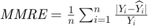 where
where  and
and  are respectively actual and estimated effort.
 - Sum Absolute Residual: summation over
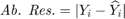
- Median (Med.) Absolute Residual: median of
- Standard deviation (SD) of Absolute Residual: standard deviation of
- Number of removed features
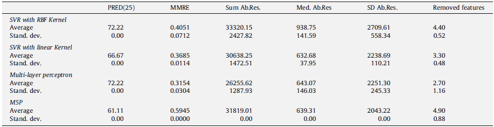
5-2) Results of Desharnais dataset
dataset = {'Desharnais'};
dataset_index = 1;
dataset_name = cell2mat(dataset);
str = sprintf('************ Our results for dataset %s:', dataset_name); disp(str);
report_experimental_results(dataset_index);
str = sprintf('************ Paper results for dataset %s:', dataset_name); disp(str);
************ Our results for dataset Desharnais:
                                               PRED25      MMRE       SumAbRes    MedAbRes    SDAbRes    RemovedFeatures
                                               ______    _________    ________    ________    _______    _______________

    SVR (RBF kernel) --> Average:              18.889       0.9329     72701      2072.3      5030.7           6
    SVR (RBF kernel) --> Stand. dev.:          3.0429     0.018434    650.02      101.33      40.697     0.70711
    SVR (linear kernel) --> Average:           44.444      0.50526     44196      1003.7      2697.4         2.6
    SVR (linear kernel) --> Stand. dev.:            0    0.0027917    599.87      38.128      87.557     0.54772
    Multi-layer perceptron --> Average:        58.889      0.53145     37328      923.73      2428.5           4
    Multi-layer perceptron --> Stand. dev.:     4.969      0.13798    6628.9      478.81      507.73           1
    M5P --> Average:                           51.111      0.57424     42068      1057.7      3037.1         4.4
    M5P --> Stand. dev.:                       2.4845      0.17723      3701      50.545      656.15      1.5166

************ Paper results for dataset Desharnais:
5-3) Results of NASA dataset
dataset = {'NASA'};
dataset_index = 2;
dataset_name = cell2mat(dataset);
str = sprintf('************ Our results for dataset %s:', dataset_name); disp(str);
report_experimental_results(dataset_index);
str = sprintf('************ Paper results for dataset %s:', dataset_name); disp(str);
************ Our results for dataset NASA:
PRED25 MMRE SumAbRes MedAbRes SDAbRes RemovedFeatures
______ _________ ________ ________ _______ _______________
SVR (RBF kernel) --> Average: 54.444 0.28048 12.008 12.008 0 0.8
SVR (RBF kernel) --> Stand. dev.: 14.098 0.045345 1.9636 1.9636 0 0.085703
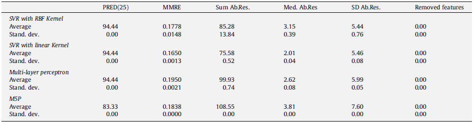
SVR (linear kernel) --> Average: 100 0.06051 2.5842 2.5842 0 0.44444
SVR (linear kernel) --> Stand. dev.: 0 0.0020549 0.051095 0.051095 0 0
Multi-layer perceptron --> Average: 100 0.010697 0.35806 0.35806 0 0.57778
Multi-layer perceptron --> Stand. dev.: 0 0.0070661 0.28696 0.28696 0 0.24036
M5P --> Average: 93.333 0.059819 1.4757 1.4757 0 0.53333
M5P --> Stand. dev.: 2.4845 0.016586 0.47804 0.47804 0 0.49496
************ Paper results for dataset NASA:
5-4) Results of COCOMO dataset
dataset = {'COCOMO'};
dataset_index = 3;
dataset_name = 'COCOMO';
str = sprintf('************ Our results for dataset %s:', dataset_name); disp(str);
report_experimental_results(dataset_index);
str = sprintf('************ Paper results for dataset %s:', dataset_name); disp(str);
************ Our results for dataset COCOMO:
                                                          PRED25      MMRE      SumAbRes    MedAbRes    SDAbRes    RemovedFeatures
                                                          ______    ________    ________    ________    _______    _______________

    dataset 1: SVR (RBF kernel) --> Average:              29.091      1.1019    9776.2      69.492      1920.5        10.2
    dataset 1: SVR (RBF kernel) --> Stand. dev.:          4.0656      0.3727    254.16      21.069      15.537      1.9235
    dataset 2: SVR (RBF kernel) --> Average:              21.818      0.8877     10394      266.23      1804.8        10.6
    dataset 2: SVR (RBF kernel) --> Stand. dev.:          4.9793     0.22195    135.96       38.15      14.604      2.9665
    dataset 3: SVR (RBF kernel) --> Average:              32.727     0.92175    3260.7      49.036      660.61         8.6
    dataset 3: SVR (RBF kernel) --> Stand. dev.:          4.9793     0.54567    366.36      36.201      25.306      2.7019
    dataset 4: SVR (RBF kernel) --> Average:                  46     0.78241    985.29      38.262      157.14         9.2
    dataset 4: SVR (RBF kernel) --> Stand. dev.:          8.9443    0.079627    75.121      12.241      8.4498      2.0494
    dataset 5: SVR (RBF kernel) --> Average:                  30      4.7492    1015.4      73.781      106.71         9.4
    dataset 5: SVR (RBF kernel) --> Stand. dev.:               0      1.3208    65.421      27.668      11.091      2.0736
    dataset 6: SVR (RBF kernel) --> Average:                  40      1.2804     12830      34.721      3498.7           8
    dataset 6: SVR (RBF kernel) --> Stand. dev.:               0     0.46777    13.308      2.9872      0.6122      1.4142
    dataset 1: SVR (linear kernel) --> Average:           32.727      1.1015    7997.3      83.009      1599.8         9.4
    dataset 1: SVR (linear kernel) --> Stand. dev.:       4.9793     0.61717      2848      33.159      670.99      2.3022
    dataset 2: SVR (linear kernel) --> Average:           45.455     0.67983    8038.1      88.858      1358.4         7.8
    dataset 2: SVR (linear kernel) --> Stand. dev.:       6.4282      0.2018    156.86      32.991       27.54     0.83666
    dataset 3: SVR (linear kernel) --> Average:           43.636      2.1905    2798.5      88.964      489.17           8
    dataset 3: SVR (linear kernel) --> Stand. dev.:       4.0656       1.175    571.17      27.583      190.52      2.1213
    dataset 4: SVR (linear kernel) --> Average:               50      1.1974    673.94      47.965      68.586         7.2
    dataset 4: SVR (linear kernel) --> Stand. dev.:       7.0711      1.2301    106.65      14.059      2.0137      1.4832
    dataset 5: SVR (linear kernel) --> Average:               38      4.3922    637.22      46.068      67.446         8.2
    dataset 5: SVR (linear kernel) --> Stand. dev.:       4.4721      2.0455    237.18       21.36      39.823        2.49
    dataset 6: SVR (linear kernel) --> Average:               60     0.82207     11002      16.198      2948.6         8.5
    dataset 6: SVR (linear kernel) --> Stand. dev.:            0    0.088915    118.23      2.7194      25.539     0.70711
    dataset 1: Multi-layer perceptron --> Average:        41.818     0.82375    8748.5      40.881      2230.3           8
    dataset 1: Multi-layer perceptron --> Stand. dev.:    4.9793     0.23007      3939      24.457      1215.3      2.1213
    dataset 2: Multi-layer perceptron --> Average:        41.818      2.6118    8027.3      301.86        1159           8
    dataset 2: Multi-layer perceptron --> Stand. dev.:    8.1312      3.2375      2545      324.24      448.53           2
    dataset 3: Multi-layer perceptron --> Average:            40      2.5933    2638.9      91.941      396.42         9.2
    dataset 3: Multi-layer perceptron --> Stand. dev.:    4.9793      1.8202    712.79      16.486       183.9      1.9235
    dataset 4: Multi-layer perceptron --> Average:            46      3.6972      1816      67.695      258.58          10
    dataset 4: Multi-layer perceptron --> Stand. dev.:    5.4772      2.7331    1006.1      10.982      209.36      1.2247
    dataset 5: Multi-layer perceptron --> Average:            40      6.7237    1266.7      62.077      183.02         7.6
    dataset 5: Multi-layer perceptron --> Stand. dev.:    7.0711      3.7419    701.01      22.505       111.4      2.6077
    dataset 6: Multi-layer perceptron --> Average:            55      2.6615    7326.5      58.926      2019.4           9
    dataset 6: Multi-layer perceptron --> Stand. dev.:    7.0711       1.996    2114.4      3.8431      806.68      2.8284
    dataset 1: M5P --> Average:                           32.727      2.8632    8597.7      120.94      1519.7         7.2
    dataset 1: M5P --> Stand. dev.:                       4.9793      1.4943    2731.3      48.614      519.28      1.9235
    dataset 2: M5P --> Average:                           30.909      1.4129    6862.9      180.66      987.43           6
    dataset 2: M5P --> Stand. dev.:                       4.9793      1.1566    2532.9      67.349      486.46      2.1213
    dataset 3: M5P --> Average:                           52.727      2.2551    2480.8      60.886      427.77        10.4
    dataset 3: M5P --> Stand. dev.:                       4.0656     0.32078    252.02      9.9901      77.327      1.6733
    dataset 4: M5P --> Average:                               48      2.0677    3339.6      50.167      618.96         7.8
    dataset 4: M5P --> Stand. dev.:                       4.4721      1.1575      2152      1.9892      445.98      2.1679
    dataset 5: M5P --> Average:                               28      3.0099    527.19        42.1      45.616           7
    dataset 5: M5P --> Stand. dev.:                       8.3666      1.9043    238.73      11.195      26.376      1.7321
    dataset 6: M5P --> Average:                               40      1.1939    9303.1      33.294      2381.7         9.5
    dataset 6: M5P --> Stand. dev.:                            0    0.062608      2010      1.6766      604.04      2.1213

************ Paper results for dataset COCOMO:
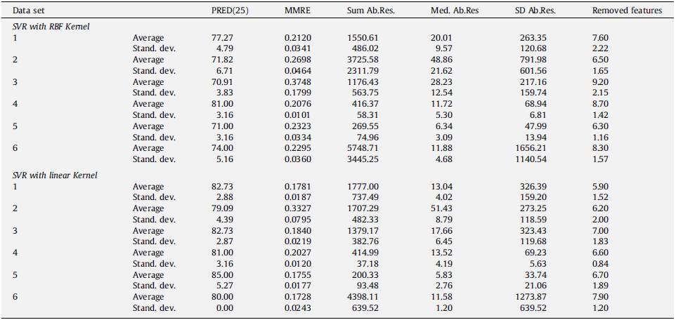
5-5) Results of Albrecht dataset
dataset = {'Albrecht'};
dataset_index = 9;
dataset_name = cell2mat(dataset);
str = sprintf('************ Our results for dataset %s:', dataset_name); disp(str);
report_experimental_results(dataset_index);
str = sprintf('************ Paper results for dataset %s:', dataset_name); disp(str);
************ Our results for dataset Albrecht:
                                               PRED25      MMRE      SumAbRes    MedAbRes    SDAbRes    RemovedFeatures
                                               ______    ________    ________    ________    _______    _______________

    SVR (RBF kernel) --> Average:              63.333     0.36713    82.917      82.917      0           4.2333
    SVR (RBF kernel) --> Stand. dev.:           4.714    0.028606    5.2316      5.2316      0          0.42426
    SVR (linear kernel) --> Average:           93.333    0.058533    28.223      28.223      0           2.6333
    SVR (linear kernel) --> Stand. dev.:       9.4281    0.033188    11.344      11.344      0          0.70711
    Multi-layer perceptron --> Average:        96.667    0.026914    24.687      24.687      0           3.1333
    Multi-layer perceptron --> Stand. dev.:     4.714    0.015524    16.172      16.172      0          0.75425
    M5P --> Average:                           86.667     0.13077    59.675      59.675      0           3.2333
    M5P --> Stand. dev.:                       9.4281      0.0378    4.7832      4.7832      0           1.0842

************ Paper results for dataset Albrecht:
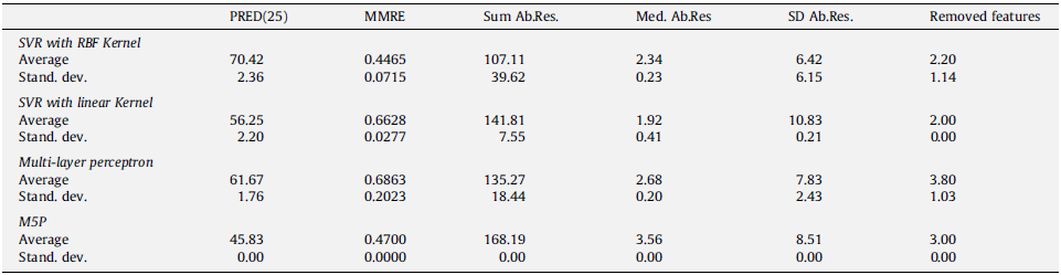
5-6) Results of Kemerer dataset
dataset = {'Kemerer'};
dataset_index = 10;
dataset_name = cell2mat(dataset);
str = sprintf('************ Our results for dataset %s:', dataset_name); disp(str);
report_experimental_results(dataset_index);
str = sprintf('************ Paper results for dataset %s:', dataset_name); disp(str);
************ Our results for dataset Kemerer:
                                               PRED25      MMRE      SumAbRes    MedAbRes    SDAbRes    RemovedFeatures
                                               ______    ________    ________    ________    _______    _______________

    SVR (RBF kernel) --> Average:              63.333     0.36713    82.917      82.917      0           4.2333
    SVR (RBF kernel) --> Stand. dev.:           4.714    0.028606    5.2316      5.2316      0          0.42426
    SVR (linear kernel) --> Average:           93.333    0.058533    28.223      28.223      0           2.6333
    SVR (linear kernel) --> Stand. dev.:       9.4281    0.033188    11.344      11.344      0          0.70711
    Multi-layer perceptron --> Average:        96.667    0.026914    24.687      24.687      0           3.1333
    Multi-layer perceptron --> Stand. dev.:     4.714    0.015524    16.172      16.172      0          0.75425
    M5P --> Average:                           86.667     0.13077    59.675      59.675      0           3.2333
    M5P --> Stand. dev.:                       9.4281      0.0378    4.7832      4.7832      0           1.0842

************ Paper results for dataset Kemerer:
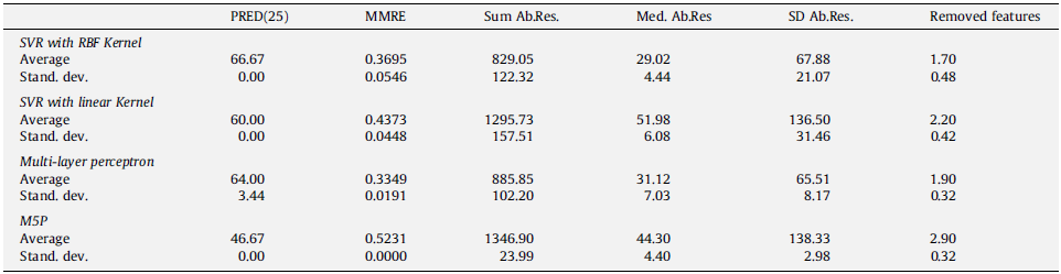
%%%%%%%%%%%%%%%%%%%%%%%%%%%%%%%%%%%%%%%%%%%%%%%%%%%%%%%%%%%%%%%
cd('./saved_files')
save workspace
cd('..')
6) ======= Analysis and Conclusions
In the following, we first analyze the time complexity of the algorithm oa paper [1] (which is not mentioned in [1]) and then we analyze and compare our obtained results and results of paper [1]. Please note that as we explain in the analysis, in many cases (but not all cases), we even outperform paper [1] and we explain the reasons.
6-1) Time complexity and settings of the proposed algorithm
The proposed algorithm in paper [1] has the following iterations and settings influencing the time cimplexity of the algorithm (these calculations are not reported in [1] and we calculate them):
- number of regression methods (denoted by
 ): paper [1] uses 4 regression methods, which are RBF SVR, linear SVR, MLP, and M5P.
 - K-fold cross validation: for some datasets it is 1-fold and for some of the datasets, it is LOOCV cross validation. We denote the number of folds by
 .
. - number of runs of GA algorithm in every fold: we denote it by
 . Subscript "a" stands for algorithm.
 - number of generations in GA algorithm: we denote it by
 . Subscript "a" stands for algorithm.
 - number of chromosomes in every generation of GA algorithm: we denote it by
 , where "a" and "C" respectvely stand for algorithm and chromosome.
Finally, the overall time complexity of the proposed algorithm in paper [1] is:  which is a very huge time complexity.
In the following, we specifically mention the original settings and the time complexity of algorithm in paper [1] for each dataset:
- Desharnais dataset [4]:
 ,
,  ,
,  ,
,  ,
,  , elitism population = ?, crossover rate = 0.8, mutation rate = 0.3 ==> = 500,000 train/test
 - NASA dataset [5]: ,
 , , , , elitism population = ?, crossover rate = 0.8, mutation rate = 0.3 ==> = 9,000,000 train/test
 - COCOMO dataset 1 [6]: , , , , , elitism population = ?, crossover rate = 0.8, mutation rate = 0.3 ==> = 500,000 train/test
- COCOMO dataset 2 [6]: , , , , , elitism population = ?, crossover rate = 0.8, mutation rate = 0.3 ==> = 500,000 train/test
- COCOMO dataset 3 [6]: , , , , , elitism population = ?, crossover rate = 0.8, mutation rate = 0.3 ==> = 500,000 train/test
- COCOMO dataset 4 [6]: , , , , , elitism population = ?, crossover rate = 0.8, mutation rate = 0.3 ==> = 500,000 train/test
- COCOMO dataset 5 [6]: , , , , , elitism population = ?, crossover rate = 0.8, mutation rate = 0.3 ==> = 500,000 train/test
- COCOMO dataset 6 [6]: , , , , , elitism population = ?, crossover rate = 0.8, mutation rate = 0.3 ==> = 500,000 train/test
- COCOMO dataset (overall) [6]:
 = 3,000,000 train/test
 - Albrecht dataset [7]: ,
 , , , , elitism population = ?, crossover rate = 0.8, mutation rate = 0.3 ==> = 12,000,000 train/test
 - Kemerer dataset [8]: ,
 , , , , elitism population = ?, crossover rate = 0.8, mutation rate = 0.3 ==> = 7,500,000 train/test
 - Korten and Gray dataset [9]: ,
 , , , , elitism population = ?, crossover rate = 0.8, mutation rate = 0.3 ==> = 8,500,000 train/test
As can be seen in the above calculations, the time complexity is very much high. According to our calculations, running the whole complete settings of the algorithm of paper [1] takes a very long time (probably weeks). Also note that, they have mentioned that they have tried different number of population size, number of generations, crossover rate, and mutation rate (mentioned in page 5 in [1]), and finally found the best settings. We guess that doing so must have taken a very huge time for them to run the whole program. As we have limitted time and experimenting exactly with the same settings is impossible until the due time, we relax the settings a little bit for all datasets except the COCOMO dataset 6 which is performed with the exact settings as in [1] (but with less number of simulations of GA). Note that even we have relaxed the settings, but it still takes a long time, for example for NASA dataset, it almost took one day to run! The settings which we choose for every dataset are listed in the following:
- Desharnais dataset [4]: , ,
 ,
,  ,
,  , elitism population = 10, crossover rate = 0.8, mutation rate = 0.3 ==> = 10,000 train/test
 - NASA dataset [5]: , , , , , elitism population = 10, crossover rate = 0.8, mutation rate = 0.3 ==> = 180,000 train/test
- COCOMO dataset 1 [6]: , , , , , elitism population = 10, crossover rate = 0.8, mutation rate = 0.3 ==> = 10,000 train/test
- COCOMO dataset 2 [6]: , , , , , elitism population = 10, crossover rate = 0.8, mutation rate = 0.3 ==> = 10,000 train/test
- COCOMO dataset 3 [6]: , , , , , elitism population = 10, crossover rate = 0.8, mutation rate = 0.3 ==> = 10,000 train/test
- COCOMO dataset 4 [6]: , , , , , elitism population = 10, crossover rate = 0.8, mutation rate = 0.3 ==> = 10,000 train/test
- COCOMO dataset 5 [6]: , , , , , elitism population = 10, crossover rate = 0.8, mutation rate = 0.3 ==> = 10,000 train/test
- COCOMO dataset 6 [6]: , ,
 , , , elitism population = 30, crossover rate = 0.8, mutation rate = 0.3 ==> = 100,000 train/test
 - COCOMO dataset (overall) [6]: = 60,000 train/test
- Albrecht dataset [7]: , , , , , elitism population = 10, crossover rate = 0.8, mutation rate = 0.3 ==> = 240,000 train/test
- Kemerer dataset [8]: , , , , , elitism population = 10, crossover rate = 0.8, mutation rate = 0.3 ==> = 60,000 train/test
- Korten and Gray dataset [9]: We did not have access to this dataset. It is not publically avaliable.
6-2) Our critiques on the paper [1]
Although paper [1] has its merits and novelty, but it has several serious flaws. Here, we mention our critiques on it:
- The base of this paper has a big un-noticed flaw which is considered as "cheating" in machine learning. They need to have a validation set in addition to training and testing sets in their data splits, to ttune the parameters. They are optimizing the parameters on the test set and finally, they report the best obtained results on the test set. The correct way is to divide the dataset into three sets, which are training, testing, and validation sets and when optimizing the parameters, the validation set should be pretended as test set. Finally, using the obtained optimum parameters, the system is trained by the train set and tested on the actual test set.
- As mentioned before, the fitness function of the proposed GA algorithm is . Notice that
 is in range [0,100] and thus the first part of fitness function, which is
  , is in range [0,100]. That is while the second part of the fitness is
  which is around the value of 0.1 or 0.01. So, the impact of the the second part is almost ignored. That is probably why they had to change the fitness function to for COCOMO dataset, although they are inspired by paper [10] which has merely used for evaluation.
 - As mentioned in section 6-1, the time complexity of the agorithm of [1] is
 which is a very huge time complexity, making it almost impractical especially when dealing with the realtime data.
 - Paper [1] has not mentioned the minimum and maximum ranges of the parameters used when converting the binary string of parameters in the chromosomes to the actual values of parameters. They have said that the user should choose it. That would be okay if they had actually report the minimum and maximum ranges of values in the experimental results. Thus, no one can reproduce their results without knowing what ranges they have used.
- Paper [1] has not mentioned the number of chromosomes they have set for the elitism replacement. Therefore, again, reproducing their exact results like them is impossible without knowing the detailed settings such as this.
- For Desharnais dataset [4], paper [1] randomly selects 18 samples out of 81 samples for test set. The remaining 63 samples are training samples. To the best of our understanding, paper [1] does not do this split for several times to take average afterwards! When the sampling is random, it is expected to sample and run for several sufficient times and take the average of the results, otherwise the results would be different in every attempt. Probably the reason that they have not dome it is that they run GA algorithm for 10 times and they give this responsibility to the runs of GA.
6-3) Analysis and comparison of the results
In the following, for each dataset, we analyze and compare the results obtained from our implementation and the results reported in the original paper [1].
Desharnais dataset [4]:
- Pred(25): Its obtained results are not completely similar to the original results. The reasons of these differences are explained at the end of section 6-3.
- MMRE: The MMRE of M5P is obtained similar to the original MMRE (considering its std) which are (0.5742 + or - 0.1772) and (0.5945 + or - 0).
- Sum Ab. Res.: Its obtained results are not completely similar to the original results. The reasons of these differences are explained at the end of section 6-3.
- Med. Ab. Res.: Its obtained results are not completely similar to the original results. The reasons of these differences are explained at the end of section 6-3.
- SD. Ab. Res.: The result of linear SVR (2697.4 + or - 87.557) is similar to its original (2251.30 + or - 110.21). Moreover, the result of MLP (2428.5 + or - 507.73) is similar to its original result (2251.30 + or - 245.33).
- Number of Removed Features: The results of linear SVM (2.6 + or - 0.5477) and MLP (4 + or - 1) and MP5 (4.4 + or - 1.5166) are respectively similar to their original results, which are (3.30 + or - 0.48), (2.70 + or - 1.16), and (4.90 + or - 0.88).
NASA dataset [5]:
- Pred(25): Its obtained results are not completely similar to the original results. The reasons of these differences are explained at the end of section 6-3.
- MMRE: For linear SVR (0.06051 + or - 0.0020), MLP (0.0106 + or - 0.0070), and M5P (0.0598 + or - 0.0165) we strongly outperform paper [1], which has results of respectively (0.1650 + or - 0.0013), (0.1950 + or - 0.0021), and (0.1838 + or - 0). The reasons of our outperformance are explained at the end of section 6-3.
- Sum Ab. Res.: For all methods, we strongly outperform paper [1]. The reasons of our outperformance are explained at the end of section 6-3.
- Med. Ab. Res.: In linear SVM (2.5842 + or - 0.0510) and MLP (0.3580 + or - 0.2869), we are close to their original results which are (2.01 + or - 0.04) and (2.62 + or - 0.08).
- SD. Ab. Res.: For all methods, we strongly outperform paper [1]. The reasons of our outperformance are explained at the end of section 6-3.
- Number of Removed Features: We have found different best number of removed features. The reasons of these differences are explained at the end of section 6-3.
COCOMO datasets 1, 2, 3, 4, 5, and 6 [6]:
- Its obtained results are not completely similar to the original results. The reasons of these differences are explained at the end of section 6-3.
Albrecht dataset [7]:
- Pred(25): Its obtained results are not completely similar to the original results. The reasons of these differences are explained at the end of section 6-3.
- MMRE: For all methods, we strongly outperform paper [1]. The reasons of our outperformance are explained at the end of section 6-3.
- Sum Ab. Res.: For all methods, we strongly outperform paper [1]. The reasons of our outperformance are explained at the end of section 6-3.
- Med. Ab. Res.: Its obtained results are not completely similar to the original results. The reasons of these differences are explained at the end of section 6-3.
- SD. Ab. Res.: For all methods, we strongly outperform paper [1]. The reasons of our outperformance are explained at the end of section 6-3.
- Number of Removed Features: We have found different best number of removed features. The reasons of these differences are explained at the end of section 6-3.
Kemerer dataset [8]:
- Pred(25): Except for RBF SVM which we have close result to the original result, we strongly outperform paper [1]. The reasons of our outperformance are explained at the end of section 6-3.
- MMRE: For all methods, we strongly outperform paper [1]. The reasons of our outperformance are explained at the end of section 6-3.
- Sum Ab. Res.: For all methods, we strongly outperform paper [1]. The reasons of our outperformance are explained at the end of section 6-3.
- Med. Ab. Res.: Its obtained results are not completely similar to the original results. The reasons of these differences are explained at the end of section 6-3.
- SD. Ab. Res.: For all methods, we strongly outperform paper [1]. The reasons of our outperformance are explained at the end of section 6-3.
- Number of Removed Features: We have found different best number of removed features. The reasons of these differences are explained at the end of section 6-3.
Korten and Gray dataset [9]:
We did not have access to this dataset. It is not publically avaliable.
The reasons of the many cases where we outperform paper [1]:
- As mentioned in item 4 of section 6-2, paper [1] has not mentioned the minimum and maximum ranges of the parameters used when converting the binary string of parameters in the chromosomes to the actual values of parameters. Thus, we have chosen some appropriate ranges for the parameters as was reported in section 4-2. The ranges of parameters we have chosen must have been better than those chosen in paper [1] (which are not reported in paper), and thus our obtained results are better.
- The GA algorithm, which is a metaheuristic optimization algorithm, has randomness and although we are running for several times and take average, but the results might differ because of randomness.
The reasons of some "slight differences" between our results and the original results are listed in the following:
- As mentioned in item 4 of section 6-2, paper [1] has not mentioned the minimum and maximum ranges of the parameters used when converting the binary string of parameters in the chromosomes to the actual values of parameters. Thus, we have chosen some appropriate ranges for the parameters as was reported in section 4-2. Therefore, the ranges of parameters, which determines the search space of the GA algorithm, might be different in paper [1] and our implementation.
- As mentioned in item 5 of section 6-2, paper [1] has not mentioned the number of chromosomes they have set for the elitism replacement. Therefore, again, reproducing their exact results like them is impossible without knowing the detailed settings such as this.
- The GA algorithm, which is a metaheuristic optimization algorithm, has randomness and although we are running for several times and take average, but the results might differ because of randomness.
- As mentioned in section 6-1 and item 3 of section 6-2, the time complexity of the agorithm of [1] is which is a very huge time complexity, making it almost impractical especially when dealing with the realtime data and makes it impossible to run with the original settings in the limitted time before the deadline. So, we have relaxed the settings of experiments a little bit as were mentioned in section 6-1. Please note that even we have relaxed the settings, but it still takes a long time, for example for NASA dataset, it almost took more than half a day to run and COCOMO6 took a complete day! Moreover, note that in some case, std of out results are higher than the original results and the reason is that we have ran the GA algorithm for less number of times because of huge time complexity.
7) ======= List of Used Files
In the following, there is a list of functions and files that we used in this project:
- Our implementation: ./main.m
- Our implementation: ./Functions/binary_GA.m
- Our implementation: ./Functions/calculate_fitness.m
- Our implementation: ./Functions/report_experimental_results.m
- For M5P regression/model tree: M5PrimeLab. It can be accessed in this URL: [11]
- For training in SVR regression: fitrsvm function. Its Mathworks document can be accessed in this URL: [12]
- For prediction in SVR regression: Its Mathworks document can be accessed in this URL: [13]
- For training MLP neural network: Its Mathworks document can be accessed in this URL: [14]
8) ======= References
[1] Adriano LI Oliveira, Petronio L. Braga, Ricardo MF Lima, and Márcio L. Cornélio. "GA-based method for feature selection and parameters optimization for machine learning regression applied to software effort estimation." information and Software Technology, vol. 52, no. 11, pp. 1155-1166, 2010.
[2] K. Vinay Kumar, Vadlamani Ravi, Mahil Carr, and N. Raj Kiran. "Software development cost estimation using wavelet neural networks." Journal of Systems and Software, vol. 81, no. 11 pp. 1853-1867, 2008.
[3] Manfred Vogel, Manfred Breit, and Fabian Märki. "Optimization of 4D Process Planning using Genetic Algorithms." 2004.
[4] http://promise.site.uottawa.ca/SERepository/datasets/desharnais.arff, Accessed: April 2018
[5] Adriano LI Oliveira. "Estimation of software project effort with support vector regression." Neurocomputing, vol. 69, no. 13-15, pp. 1749-1753, 2006
[6] http://promise.site.uottawa.ca/SERepository/datasets/cocomo81.arff, Accessed: April 2018
[7] https://zenodo.org/record/268467#.WqhS0G3waUk, Accessed: April 2018
[8] https://zenodo.org/record/268464#.WqhUWm3waUk, Accessed: April 2018
[9] Chikako Van Koten and A. R. Gray. "Bayesian statistical effort prediction models for data-centred 4GL software development." Information and Software Technology, vol. 48, no. 11, pp. 1056-1067, 2006.
[10] Iris Fabiana de Barcelos Tronto, José Demísio Simões da Silva, and Nilson Sant’Anna. "An investigation of artificial neural networks based prediction systems in software project management." Journal of Systems and Software, vol. 81, no. 3, pp. 356-367, 2008.
[11] http://www.cs.rtu.lv/jekabsons/regression.html, Accessed: April 2018
[12] https://www.mathworks.com/help/stats/fitrsvm.html, Accessed: april 2018
[13] https://www.mathworks.com/help/stats/compactclassificationsvm.predict.html, Accessed: April 2018
[14] https://www.mathworks.com/help/nnet/ref/fitnet.html, Accessed: April 2018