Optimization of Steering Linkages
In this project, a steering linkage is designed. This linkage is designed to control the angles of the front wheels of a car. The Ackermann steering condition defines the optimal relationship between the angles of the two front wheels of a car. The linkage should control the wheels of the car to best match with this condition.
Project Prepared by: Katie DiCola, for ECE-602 final project, April 2018
Contents
Ackermann condition
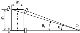
The Ackermann condition gives a mathematical definition of the ideal angles of the wheels when steering a car. The wheels should not be parallel (as one might expect) but rather must satisfy this condition, which is shown in this image:
The equation relating the outer wheel angle,  , and inner wheel angle,
  is:
is:
Where  is a normalized expression of the wheel base divided by the wheel track,
  .
.
Linkage Design
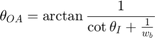
This can be represented with different kinds of linkages. Typically, a six-bar linkage is used with a rack-and-pinion steering control. This is shown in the following image. In this case, only the central take-off case is analyzed. (The side take-off case can be normalized such that it is identical to the central take-off case.)
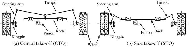
A kinematic diagram of the linkage is shown here:
Note that we are designing the linkage to be symmetrical, thus  is the steering arm length and
  is the tie rod length.
Link Length Optimization
No linkage will be able to perfectly represent the Ackermann condition. Instead, an optimization is performed to determine a linkage which matches as closely as possible. Here, the desired closest match is the linkage with the smallest maximum steering error over a range of input angles.
So, our optimization problem is:
Minimize the maximum steering error over a given range of angles, subject to the condition that the linkage is still kinematically feasible.
The maximum steering error,  , for any given set of angles, , is:

Therefore, our objective function is:

And the constraints are:


Which are all non-linear inequality constraints that are meant to ensure that the resulting linkage is kinematically feasible. The equations that define these  values are given in the original paper. The functions that implement them are given in the "Constraint Functions" section. There is an additional constraint that
  must remain monotone throughout the angular movement. Because of the format of the input/output angles this will always be true for monotone
  starting at 0 within our limits (i.e. when
  , then
  and b will increase or decrease with ).
CODE: Initialization
Define the wheel track, wheel base, the distance between the rack & the axis of the kingpins, and the set of angles over which the optimization is performed.
wt = 1;
wb = 1.4;
h = 0.1;
thetain = 0:0.1:60;
thetain = thetain*pi/180;
CODE: Minimization
Because we have a nonlinear objective function and nonlinear constraint functions, we use "fmincon":
The objective function "sterr" and the constraint function "cnst_func" are both given in the sections below.
(Note: The output is displayed at the end of the objective function section of the document rather than here due to a known MATLAB bug)
First, we define a secondary function, vsterr, so that the parameters wt, h, and wb can be passed to sterr without including them in the optimization:
vsterr = @(x)(sterr(thetain,x(1),x(2),wt,h,wb));
Now, we use fmincon with the following options:
The starting point is a known feasible point  and
and  .
.
Lower bound of both link lengths is zero, as link lengths cannot be negative.
Upper bound is set to 10. This was chosen as an arbitrarily high number - 10 times the wheel track. Link lengths should never reach this number.
The constraint function is written as with the @(x) to pass  ,
,  , and to the function without including them in the optimization.
x = fmincon(vsterr,[0.2 0.4],[],[],[],[],[0 0],[10 10],@(x)cnst_func(x,h,wt,thetain));
la_opt = x(1);
lt_opt = x(2);

disp(['The optimized steering arm length is ' num2str(la_opt) ' and the optimized tie bar length is ' num2str(lt_opt)]);
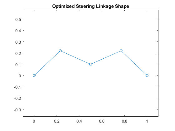
CODE: Plotting the resulting linkage
The linkage will be plotted to check if it is practical.
la = la_opt;
lt = lt_opt;

% Find the input/output angles at b = 0.
b = 0;
k1 = -lt^2 + la^2 + h^2;
k2 = (k1 + (wt/2 + b)^2)/la;
delta1 = 4*h^2 - k2^2 + (wt+2*b)^2;
z1 = (2*h + sqrt(delta1))/(k2+wt+2*b);
stheta1 = 2*z1/(1+z1^2);
ctheta1 = (1-z1^2)/(1+z1^2);
theta1 = atan2(stheta1,ctheta1);

% When b = 0, linkage is symmetrical.
theta6 = theta1;

% Link end locations:
xlink = zeros(6,1);
ylink = zeros(6,1);

xlink(1) = 0;
ylink(1) = 0;

xlink(2) = xlink(1) + la*cos(theta1);
ylink(2) = ylink(1) + la*sin(theta1);

xlink(3) = wt/2;
ylink(3) = h;

xlink(4) = xlink(3);
ylink(4) = ylink(3);

xlink(5) = wt - xlink(2);
ylink(5) = ylink(2);

xlink(6) = wt;
ylink(6) = 0;

% Plot the optimized linkage shape:
plot(xlink,ylink,'-o'); axis equal; xlim([-0.1 1.1]);
title('Optimized Steering Linkage Shape');
CODE: Objective Function
This function gives the maximum steering error, . The inputs are the two optimization variables ( and
and  ), the vector of angles over which the optimization is performed (), and the additional values that define the linkage (, , and ).
function phi = sterr(thetain,la,lt,wt,h,wb)

% Find "theta0" - the angle between horizontal and steering arm when b = 0.
b = 0;
k1 = -lt^2 + la^2 + h^2;
k2 = (k1 + (wt/2 + b)^2)/la;
delta1 = 4*h^2 - k2^2 + (wt+2*b)^2;
if delta1 < 0
    % The linkage is not feasible.
    phi = NaN;
    return
end
z1 = (2*h + sqrt(delta1))/(k2+wt+2*b);
stheta1 = 2*z1/(1+z1^2);
ctheta1 = (1-z1^2)/(1+z1^2);
theta0 = atan2(stheta1,ctheta1);

% Our current input angles are the angles of the wheel, which must be converted
% to be the angles of the steering arm by subtracting them from theta0.
thetain = theta0 - thetain;

% For each angle, determine the output angle of the linkage and the desired
% output angle from the Ackermann condition.
theta6 = zeros(1,length(thetain));
theta6a = zeros(1,length(thetain));
for i = 1:length(thetain)
    theta1 = thetain(i);

    % Linkage output angle is calculated:
    k1 = -lt^2 + la^2 + h^2;
    delta = la^2*cos(theta1)^2 - k1 + 2*la*h*sin(theta1);
    b = la*cos(theta1) - wt/2 + sqrt(delta);

    k3 = (k1 + (wt/2 - b)^2)/la; % ORIGINAL PAPER HAS ERROR IN THIS EQUATION. originally (k1 - (wt/2 ...
    delta6 = 4*h^2 - k3^2 + (wt-2*b)^2;
    if delta<0 || delta6<0
        theta6(i) = 0;
        theta6a(i) = 0;
    else
        z6 = (2*h + sqrt(delta6))/(k3+wt-2*b);
        stheta6 = 2*z6/(1+z6^2);
        ctheta6 = (1-z6^2)/(1+z6^2);
        theta6(i) = atan2(stheta6,ctheta6);

        % Ackermann condition output angle is calculated:
        theta6a(i) = atan(1/(cot(theta1) + (1/wb)));
    end
end
% Convert from the steering arm angles to wheel angles.
theta6 = theta6 - theta0;

% Maximum steering error:
phi = max(abs(theta6-theta6a));
end
CODE: Constraint functions
All constraint functions are managed using "cnst_func" There are three nonlinear inequality constraints. The format of these constraints is  , so we set
  to enforce
  . There are no equality constraints.
function [c, ceq] = cnst_func(x,h,wt,thetain)
c = [-delta10func(x(1),x(2),h,wt) -deltaat60func(x(1),x(2),h,wt) -delta6func(thetain,x(1),x(2),h,wt)];
ceq = [];
end
Each individual constraint function is given below.
This function verifies that the linkage is kinematically feasible:
function d10 = delta10func(la, lt, h, wt)
k1 = -lt^2 + la^2 + h^2;
k2 = (k1 + (wt/2)^2)/la;
d10 = 4*h^2 - k2^2 + wt^2;
end
This function verifies that the input link is able to rotate the full amount:
function D = deltaat60func(lt,la,h,wt)
thetain = 60*pi/180;

b = 0;
k1 = -lt^2 + la^2 + h^2;
k2 = (k1 + (wt/2 + b)^2)/la;
delta1 = 4*h^2 - k2^2 + (wt+2*b)^2;
if delta1 < 0
    D = NaN;
    return
end
z1 = (2*h + sqrt(delta1))/(k2+wt+2*b);
stheta1 = 2*z1/(1+z1^2);
ctheta1 = (1-z1^2)/(1+z1^2);
theta0 = atan2(stheta1,ctheta1);

thetain = thetain - theta0;

k1 = -lt^2 + la^2 + h^2;
D = la^2*cos(thetain)-k1+2*la*h*sin(thetain);
end
This function verifies that the output link is always able to rotate with the input link.
function D = delta6func(thetain,la,lt,h,wt)
D = zeros(1,length(thetain));
for i = 1:length(thetain)
    theta1 = thetain(i);
    k1 = -lt^2 + la^2 + h^2;
    delta = la^2*cos(theta1)^2 - k1 + 2*la*h*sin(theta1);
    b = la*cos(theta1) - wt/2 + sqrt(delta);
    k3 = (k1 + (wt/2 - b)^2)/la;
    D(i) = 4*h^2 - k3^2 + (wt - 2*b)^2;
end
end
Local minimum found that satisfies the constraints.

Optimization completed because the objective function is non-decreasing in
feasible directions, to within the default value of the optimality tolerance,
and constraints are satisfied to within the default value of the constraint tolerance.


The optimized steering arm length is 0.31848 and the optimized tie bar length is 0.29438