Storey-based lateral stability of unbraced steel frames subjected to variable loading
Terence Ma ID: 20462378
Contents
- 1. Introduction
- 2. Original Problem
- 3. Further Reformulation
- 4. Discussion of Convexity
- 5. Proposed Solution
- 6. Data Sources
- 7. Nesterov Method Implementation
- 8. Convergence
- 9. fmincon Implementation
- 10. Conclusion
- References
- Appendix A1. Plotting the second derivative of

- Appendix A2. Steepest Descent Algorithm
- Appendix A3. Gradient Descent Algorithm
- Appendix A4. Nesterov Scheme Algorithm
- Appendix A5. fmincon Objective Function
1. Introduction
This paper presents an optimization problem for determining the minimum structural loading combinations which will result in the instability of a storey steel frame. The proposed optimization problem was originally presented in Xu et. al. (2001) and modified in Xu (2003). Xu (2003) reformulates the problem in the form of a non-linear optimization problem. This paper solves solves the Xu (2003) problem using various optimization methods, and the results are compared with the original.
2. Original Problem
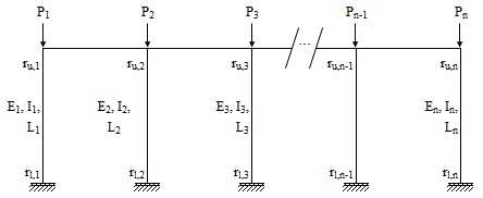
Consider the case of a storey steel frame with  columns, shown in the figure below.
Let  be the indices of the
  columns in the frame. Then
  ,
,  ,
,  , and
, and  are the axial load, modulus of elasticity, moment of inertia, and length of each column. Let
 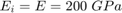 for all members. All member end connections are idealized rotational springs with end fixity factors
  and
and  representing the resistance to rotation at the upper and lower connections of the columns, respectively. An end fixity factor of zero indicates a pinned connection, while an end fixity factor of unity represents a fixed connection. Note that the end fixity factors depend on the properties of the members that are attached to the respective connections (i.e. the beams).
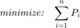
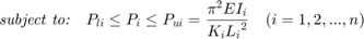
Now, there are many different combinations of loads that can cause the frame to become laterally unstable. The goal of the optimization problem is to determine the most critical combination of loads that would cause instability. This is done by minimizing the total load while specifying the instability criterion of the frame as an equality constraint. A box constraint is also applied to the forces on the columns. The original problem is shown below (Xu et al., 2001):

where  is the lateral stiffness of the frame as a whole,
  is the lateral stiffness of each column, and
  indicates that the frame has become unstable.
  is typically taken as zero and is the lower bound axial load. If
  is exceeded, the column would experience rotational buckling failure. Thus, is an upper bound for each optimization variable.
  is the column effective length factor and is computed as a function of the end fixity factors (Xu, 2003). Finally,
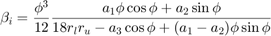
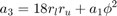
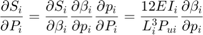
  is a non-linear function of the optimization variable and end fixity factors, presented as follows:

![$$a_1 = 3[r_l(1-r_u)+r_u(1-r_l)]$$](ECE_602_Project_Terence_Ma_20462378_eq03082575743518368342.png)

Clearly, the equality constraint is non-linear due to the non-linearity of with respect to each optimization variable. Note that values of may be positive or negative. A negative value of indicates that the column has lost all of its lateral stiffness and must rely on the lateral stiffness of the other columns in order to remain standing.
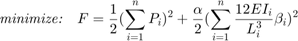
The solution of the original problem with the non-linear equality constraint can be difficult. As such, Xu (2003) proposed a reformulation to the original problem by moving the equality constraint into the objective function, and expressing it as a penalty term, shown below:

where  is a penalty factor specified by the user. As such, the equality constraint is removed and a boxed domain can be searched to find the optimal solution.
Note also that the total load can also be maximized by multiplying the objective function by -1. This is also discussed by Xu et al. (2001) and Xu (2003) but the solution procedure is identical. Thus, this paper will only focus on the minimization problem.
3. Further Reformulation
In this paper, the modified problem presented by Xu (2003) containing the penalty factor is further reformulated. The scope of the project includes coding a gradient-based method in MATLAB in order to solve the optimization problem. The method is then tested to see if it can reproduce the results of a numerical example presented in Xu (2003). As an additional exercise, the fmincon solver from MATLAB's optimization toolbox is also utilized to compare results.
As the goal of the project is to use gradient-based methods, it was quickly noted that the formulation proposed by Xu (2003) yields discontinuous partial derivatives with respect to when the overall lateral stiffness is zero, i.e.  . In other words, the subgradient of the objective function with respect to S is a non-unique set at . To rectify this issue, an equivalent reformulation of the problem is presented below, and will be used throughout the rest of the paper.
The optimization variable is still 

 , and the optimal solution,
  , of this problem, will be the same as that of both of the previous formulations, except for small tolerance errors related to the penalty term. The penalty term disappears when approaches zero, and
  represents a desired tolerance related to the magnitude of the penalty term. Setting higher values of will result in larger penalties for small values of , which ultimately leads to a better approximation of the optimal solution of the original problem. However, increase generally makes convergence slower. Note that the first term in the objective function was also modified in order to make the objective function more sensitive to changes in the actual total force.
Note also that the modified problem is similar in form to the Lagrangian dual. However, the minimization of the Lagrangian over is a difficult problem due to the non-linearity of with respect to  .
.
4. Discussion of Convexity
The global convexity of the reformulated problem is not guaranteed. Although the problem was initially (near the beginning of this project) thought to be convex, more investigation was conducted and it was found that the problem is only convex within some portions of the domain. As such, it was much later confirmed that a global optimum is not guaranteed using the methods in this paper. Due to the complexity of the lateral stiffness equation, the problem could not be reformulated in such a way that would make it completely convex. This section explains the work that was done to investigate the convexity of the problem.
Recall that if a function  is differentiable, then it is convex over some convex subdomain if for all points in the subdomain,
  . Also, the sum of two convex functions is convex.
The Hessian of the first term in the objective function  with respect to is:
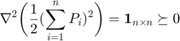
Thus, the first term in the objective function is convex. Next, the Hessian of the penalty term is shown as follows:

![$${\textit{where}\quad} \nabla S = \bigg[ \frac{\partial S_1}{\partial P_1}, \frac{\partial S_2}{\partial P_2}, ..., \frac{\partial S_n}{\partial P_n} \bigg]^T $$](ECE_602_Project_Terence_Ma_20462378_eq11579249274775153086.png)
Of course, if the Hessian of the penalty term was positive-semidefinite, then the objective function would be convex. Additionally, the domain is problem is bounded using box constraints, so the domain is convex. Now, it can be shown that:
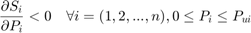
which makes intuitive sense as the application of additional axial load always reduces the lateral stiffness of the column. It was also discovered that:
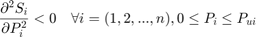
This can be shown by expressing in terms of only  , , and in the following equation, and then plotting the second derivative of over the domain
 ![${r_{u,i}, r_{l,i}} \in [0,1]\times[0,1]$](ECE_602_Project_Terence_Ma_20462378_eq10253434305944558922.png) . Recall that
. Recall that  is a function of only and .

The second derivative of with respect to  is apparently independent of , and is therefore only a function of and . Plotting over the domain gives the following surface:

The code for plotting this surface can be found in Appendix A1. Since the second derivative of is always negative, it follows from the chain rule that:

Thus, the Hessian of the penalty term is guaranteed to be positive semi-definite if the overall lateral stiffness,  . If is positive, the Hessian of the penalty term will still be positive semi-definite if is small, i.e. when the penalty function is near zero. Therefore
  , i.e. the optimization problem is guaranteed to be convex in the areas of the domain where or
  is sufficiently small. However, for
  it is unknown whether or not the objective function is convex. To further complicate the problem, it is now believed that the set of satisfying is not a convex set, so a global minimum solution is not guaranteed.
5. Proposed Solution
Over the course of the project, multiple gradient-based descent algorithms have been implemented in attempts to solve the given minimization problem. At first, the CVX toolbox for MATLAB was used, but produced an error as the penalty function contained sines and cosines, which rendered the problem inadmissible to the CVX solver. The problem is not fully convex anyway, so it would not make sense to use CVX. Secondly, the Steepest Descent and Gradient Descent methods were implemented, but they converged too slowly to prove useful. As extra information, the codes for these methods are included in Appendices A2 and A3, respectively. Upon discussion with the course professor, it was found that the Nesterov scheme (1983) may be suitable for this problem. As such, the Nesterov scheme was chosen for implementation. It is similar to the other gradient-based methods except that it varies the step size in each iteration so that the convergence efficiency is maximized. As a minor extension to the project, the fmincon solver from the MATLAB Optimization Toolbox was also implemented to solve the same problem.
One minor modification was made to the original Nesterov sceheme. The original method was written for unconstrained minimization problems. Since the current problem has box constraints, a modification was made such that if an iteration of the optimization variable exceeds the limits of the box constraint, the iteration will attempt to restart with a smaller step size until a new iterate is found to be within the limits.
Given the convexity considerations in the previous section, the first trial point in each example was selected such that it satisfied , thereby guaranteeing that some solutions with exist in the same convex search region (this was shown in the previous section). Still, however, since the set of solutions satisfying may not be a convex set, only a locally optimum value is guaranteed, and the global optimum may not always be found.
6. Data Sources
This paper replicates the results of the numerical example presented in Xu (2003). The example contains four different frames, which are identical except that the end fixity factors of the columns vary for each frame. The optimization problem is solved for all four frames using the Nesterov scheme.
The following column data was entered. All of the data was copied directly from Section 5, Tables 1 and 2 in Xu (2003).
n = 5;                                  % Number of columns
E = 2E11    *ones(n,1);                 % Modulus of elasticity (N/m2)
I = 1E-6*[129 34.1 34.1 34.1 129];      % Moment of inertia (m4)
L = 4.877   *ones(n,1);                 % Length (m)
rl = [1.0   1.0   1.0   1.0   1.0  ;    % Lower end fixity - Frame 1 (-)
      0.0   0.0   0.0   0.0   0.0  ;    % Lower end fixity - Frame 2 (-)
      1.0   1.0   1.0   1.0   1.0  ;    % Lower end fixity - Frame 3 (-)
      0.0   1.0   1.0   1.0   0.0] ;    % Lower end fixity - Frame 4 (-)
ru = [0.717 0.950 0.950 0.950 0.717;    % Upper end fixity - Frame 1 (-)
      0.717 0.717 0.717 0.717 0.717;    % Upper end fixity - Frame 2 (-)
      0.0   0.0   0.0   0.0   0.0  ;    % Upper end fixity - Frame 3 (-)
      0.0   0.0   0.0   0.0   0.0] ;    % Upper end fixity - Frame 4 (-)
Pl = [0.1   0.1   0.1   0.1   0.1] ;    % Lower bound axial force (N)
                                        %   Note: avoid Pi = 0, which
                                        %   causes divide-by-zero errors
Pu = 1E3*...
     [24495 7420  7420  7420  24495;    % Upper bound axial force - Frame 1 (N)
      14891 4511  4511  4511  14891;    % Upper bound axial force - Frame 2 (N)
      17610 4655  4655  4655  17610;    % Upper bound axial force - Frame 3 (N)
      10706 4655  4655  4655  10706];   % Upper bound axial force - Frame 4 (N)
Note that upon investigation, the values of Pu were incorrectly calculated in Xu (2003). However, for the sake of being able to compare results, the values reported in the paper will be used anyway.
7. Nesterov Method Implementation
Initial trial solutions were chosen arbitrarily and a penalty factor of  was selected. The use of was selected based on experimenting with the Nesterov algorithm for this problem.
P0 = 1E3*...
    [5000   5000    5000    5000    5000;
     1000   4000    1500    500     1000;
     1000   4000    1500    500     1000;
     2000   2000    2000    3000    2000];
alpha = 1E5;
maxiter = 2000;
As discussed previously, it was ensured that all of the initial guesses satisfy in  . The code for the function Nesterov_Method() is provided in Appendix A4. It is implemented using the following code to solve for the optimal solutions in all four frames:
opt_soln = zeros(4,n); % Store optimal solution
opt_sum = zeros(n);    % Store the total force in the optimal solution
opt_Sval = zeros(n);   % Check the stiffness of the optimal solution
conv_obj = {};         % Convergence data - penalty function
conv_pen = {};         % Convergence data - penalty function
for frame = 1:4
    [P_hist, F_hist, penalty_hist] = ...
        Nesterov_Method(P0(frame,:)',E,I,L,rl(frame,:),ru(frame,:),...
            alpha,Pl,Pu(frame,:),maxiter);
    opt_soln(frame,:) = P_hist(length(P_hist(:,1)),:);
    opt_sum(frame) = sum(opt_soln(frame,:));
    [opt_S,~] = Get_S_info(opt_soln(frame,:)',E,I,L,rl(frame,:),ru(frame,:));
    opt_Sval(frame) = sum(opt_S);
    conv_obj(frame,:) = {F_hist};
    conv_pen(frame,:) = {penalty_hist};
end
The optimal solutions for the frames as obtained from the Nesterov scheme are tabulated as follows. Note that to analyze all four frames the total runtime was about 1.5 hours.
opt_soln = opt_soln./1000; % express in kN
opt_Sval = opt_Sval./1000; % express in kN/m
fprintf('-----------------------------------------------------------------------------\n')
fprintf('          P1 (kN)   P2 (kN)   P3 (kN)  P4 (kN)  P5 (kN)  Total (kN)  S (kN/m)\n')
fprintf('-----------------------------------------------------------------------------\n')
for frame =1:4
fprintf('Frame %.0d: %5.0f   %8.0f  %8.0f  %8.0f %8.0f  %9.0f %9.1f\n',...
        frame, opt_soln(frame,1), opt_soln(frame,2), opt_soln(frame,3),...
        opt_soln(frame,4), opt_soln(frame,5), sum(opt_soln(frame,:)), ...
        opt_Sval(frame));
end
fprintf('-----------------------------------------------------------------------------\n')
-----------------------------------------------------------------------------
          P1 (kN)   P2 (kN)   P3 (kN)  P4 (kN)  P5 (kN)  Total (kN)  S (kN/m)
-----------------------------------------------------------------------------
Frame 1:   716       7420      7420      7420      716      23691       0.9
Frame 2:   504       3323      1008         0      504       5339       0.2
Frame 3:   500       4350      1058         0      500       6407       0.2
Frame 4:     0        374       374      1357        0       2106       0.1
-----------------------------------------------------------------------------
These results are compared to the ones reported by Xu (2003):
fprintf('-------------------------------------------------------------------\n')
fprintf('          P1 (kN)   P2 (kN)   P3 (kN)  P4 (kN)  P5 (kN)  Total (kN)\n')
fprintf('-------------------------------------------------------------------\n')
fprintf('Frame 1     717      7420      7420      7420      717      23694  \n')
fprintf('Frame 2       0         0         0      4485        0       4855  \n')
fprintf('Frame 3       0      1244         0      4655        0       5899  \n')
fprintf('Frame 4       0         0         0      2047        0       2047  \n')
fprintf('-------------------------------------------------------------------\n')
-------------------------------------------------------------------
          P1 (kN)   P2 (kN)   P3 (kN)  P4 (kN)  P5 (kN)  Total (kN)
-------------------------------------------------------------------
Frame 1     717      7420      7420      7420      717      23694
Frame 2       0         0         0      4485        0       4855
Frame 3       0      1244         0      4655        0       5899
Frame 4       0         0         0      2047        0       2047
-------------------------------------------------------------------
Only the results for Frame 1 match those found on Table 3 of Xu (2003). For Frames 2, 3 and 4, local minimum solutions were found, although they are still within about 10% of the global optimum indicated by Xu (2003). For these frames the solver is terminated due to one of the column loads reaching the lower bound of zero. In such a case, since the descent direction is towards the boundary of the domain, there is no choice but to get as close to the boundary as possible, stop the operation and report the local optimum values. Note that the frame stiffness for each of the solutions is virtually zero, which is expected. If a higher value of was selected, then the values of in the optimal solutions would have to be even closer to zero (the penalty would be greater for the same value of non-zero ). Moreover, it appears that the choice of trial solution has a significant effect on the results, as the relative magnitudes of the forces in the local optimum solution are similar to those of the initial guess. That is, although not always the case, if the initial guess contains a small value for a certain column, its force in the local minimum will be relatively small (if not zero). In contrast, if a certain column is assigned a large force in the trial guess, its force in the optimal solution will likely be relatively large. As such, if this project were to be repeated, it would be worth investigating the use of multi-start algorithms, and/or perhaps a different solver can be utilized.
Note that the Table 3 results in Xu (2003) also inlude maximum and proportional loading cases, which are neglected in this study. As previously mentioned, the maximization problem can easily be formulated by multiplying the objective function by -1. Similarly, the proportional loading case is easily obtained by reducing the number of optimization variables to 1 and setting all the loads in to be proportional.
8. Convergence
For each frame, the convergence of the Nesterov Method over the number of iterations was investigated. The following two figures plot the convergence of the objective function and penalty term, respectively, on a log-log scale.
figure
for frame=1:4
    subplot(2,2,frame)
    F_hist = conv_obj{frame,1};
    iters = 1:length(F_hist);
    loglog(iters,F_hist);
    title({['Objective Function, Frame ' num2str(frame)] ''});
    xlabel('Iteration #'); ylabel('F')
end
snapnow
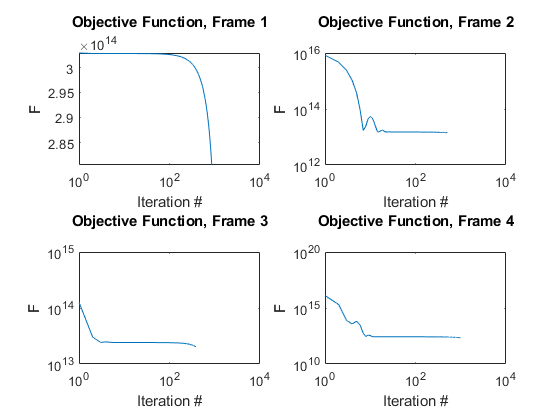
figure
for frame=1:4
    subplot(2,2,frame)
    pen_hist = conv_pen{frame,1};
    iters = 1:length(pen_hist);
    loglog(iters,pen_hist);
    title({['Penalty Term, Frame ' num2str(frame)] ''});
    xlabel('Iteration #'); ylabel('F')
end
snapnow
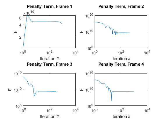
The objective function generally decreases to the optimum value over time. Note that in Frame 1 the problem began to converge more rapidly as the iterations progressed, until the interior columns reached their upper bound limit and the solver was forced to stop, yielding the correct global minimum solution. Note that Nesterov (1983) states that the solver does not guarantee a monotone decrease in the objective function, which is observed in the above figures. However, the solver eventually converges. The penalty function approaches zero, but does not reach exactly zero so long as it is small enough to not significantly affect the value of the objective function. For each frame, the penalty term was observed to gradually decrease until it reached a certain value where it did not significantly affect the objective function. Note that a magnitude of  in the penalty term is considered neligible when compared to the magnitude of the objective function (about
  ). Especially since the lateral stiffness is computed in units of Newtons per meter (N/m), penalty values in the range of represent near-zero lateral stiffness of the frame.
9. fmincon Implementation
In addition to the Nesterov scheme, the fmincon solver from the MATLAB Optimization Toolbox was used to solve the same optimization problem. The code for implementing fmincon is shown below. Note that the objective function used in this application of fmincon is included in Appendix A5.
A = []; B = []; Aeq = []; Beq = []; nonlcon = [];
options = optimoptions('fmincon', 'Algorithm', 'sqp', 'Display', 'off', ...
    'MaxFunctionEvaluations', 10000, 'MaxIterations', 1000, ...
    'FunctionTolerance', 1e-6, 'ConstraintTolerance', 1e3, 'StepTolerance', 1e-8);
opt_soln = zeros(4,n); % Store optimal solution
opt_sum = zeros(n);    % Store the total force in the optimal solution
opt_Sval = zeros(n);      % Check the stiffness of the optimal solution
for frame = 1:4
    X0 = P0(frame,:)';
    [X, Fval, ef, output, lambda] = ...
          fmincon(@(X) obj_function(X,E,I,L,rl(frame,:),ru(frame,:),alpha), X0, ...
          A,B,Aeq,Beq,Pl,Pu(frame,:),nonlcon,...
          options);
    [opt_S,~] = Get_S_info(X,E,I,L,rl(frame,:),ru(frame,:));
    opt_soln(frame,:) = X';
    opt_sum(frame) = sum(X);
    opt_Sval(frame) = sum(opt_S);
end
The optimal solutions for the frames as obtained from fmincon are tabulated as follows. Note that to analyze all four frames using fmincon the total runtime was about 15 minutes.
opt_soln = opt_soln./1000; % express in kN
opt_Sval = opt_Sval./1000; % express in kN/m
fprintf('-----------------------------------------------------------------------------\n')
fprintf('          P1 (kN)   P2 (kN)   P3 (kN)  P4 (kN)  P5 (kN)  Total (kN)  S (kN/m)\n')
fprintf('-----------------------------------------------------------------------------\n')
for frame =1:4
fprintf('Frame %.0d: %5.0f   %8.0f  %8.0f  %8.0f %8.0f  %9.0f %9.1f\n',...
        frame, opt_soln(frame,1), opt_soln(frame,2), opt_soln(frame,3),...
        opt_soln(frame,4), opt_soln(frame,5), sum(opt_soln(frame,:)), ...
        opt_Sval(frame));
end
fprintf('-----------------------------------------------------------------------------\n')
-----------------------------------------------------------------------------
          P1 (kN)   P2 (kN)   P3 (kN)  P4 (kN)  P5 (kN)  Total (kN)  S (kN/m)
-----------------------------------------------------------------------------
Frame 1:     0       7420      7420      7420     1430      23690       1.0
Frame 2:     0          0         0      4088        0       4088       0.0
Frame 3:     0       4655         0      1243        0       5898       0.2
Frame 4:     0          0      2047         0        0       2047       0.1
-----------------------------------------------------------------------------
The results from fmincon are similar to those reported by Xu (2003). The only major difference is in Frame 1, where the axial forces on the exterior columns are not equal. However, roughly the same total force is achieved as the solution for Frame 1 in Xu (2003). Clearly, fmincon is able to solve the optimization problem more accurately and efficiently compared to the Nesterov algorithm.
10. Conclusion
This paper has investigated the use of various gradient-based optimization algorithms towards the solving of a reformulated non-linear constrained optimization problem in the field of structural engineering. The problem was defined by Xu (2003) and reformulated in this paper for use with gradient-based searching algorithms. The problem was made difficult due to the non-linearity and non-convexity of the lateral stiffness constraint, which was transformed into a penalty term in the objective function. It was found that none of the CVX, Steepest Descent, or Gradient Descent methods could solve the optimization problem. The Nesterov scheme was coded and is the main focus of this project. It correctly identified the global minimum in the case of one out of four numerical examples. In the other three examples, the Nesterov scheme was unsuccessful due to the presence of local minima, but was within 10% of the global optimum. A brief analysis was conducted regarding the convergence of the Nesterov scheme over its iterations. Finally, the fmincon solver was used in MATLAB, which converged to the global minimum in all of the examples tested.
References
- Nesterov, Y.E. (1983). A method of solving a convex programming problem with convergence rate O(1/k2). Soviet Mathematics Doklady, 27(2), pp. 372-376.
- Xu, L., Liu, Y., Chen, J. (2001). Stability of unbraced frames under non-proportional loading. Structural Engineering and Mechanics(South Korea), 11(1), pp 1-16.
- Xu, L. (2003). A NLP approach for evaluating storey-buckling strengths of steel frames under variable loading. Structural and Multidisciplinary Optimization, 25(2), pp 141-150.
Appendix A1. Plotting the second derivative of
function plot_d2b()

    syms xt phi a1 a2 a3 bi rl ru K PI;
    bi = phi^3/12 * (a1*phi*cos(phi) + a2*sin(phi)) /...
        (18*rl*ru - a3*cos(phi) + (a1-a2)*phi*sin(phi));
    bi = subs(bi,a3,18*rl*ru + a1*phi^2);
    bi = subs(bi,a2, 9*rl*ru- (1-rl)*(1-ru)*phi^2);
    bi = subs(bi,a1,3*(rl*(1-ru) + ru*(1-rl)));
    bi = subs(bi,phi, sqrt(xt)*PI/K);
    bi = subs(bi,K,sqrt( (PI^2 + (6-PI^2)*ru)*(PI^2 + (6-PI^2)*rl) / (...
              (PI^2 + (12-PI^2)*ru)*(PI^2 + (12-PI^2)*rl)  ) ) );
    bi = subs(bi,PI, pi);
    dbdxt = diff(bi,xt);
    db2dxt = diff(dbdxt,xt); % Second derivative of beta_i

    npts = 10;
    ru_vec = linspace(0,1,npts);
    rl_vec = linspace(0,1,npts);
    d2bdx2 = zeros(npts,npts);
    x = 0.5; % Note: Trying any value of x from 0 to 1 gives the same result
    for i=1:npts
        for j=1:npts
            d2bdx2(i,j) = double(subs(db2dxt,...
                [xt,ru,rl],[x, ru_vec(i), rl_vec(j)]));
        end
    end
    surf(ru_vec,rl_vec,d2bdx2);
    title('$$\frac{\partial^2 \beta}{\partial p_i^2}$$','interpreter','latex');
    xlabel('r_{l,i}'); ylabel('r_{u,i}');
    xlim([0 1]); ylim([0 1]);
end
Appendix A2. Steepest Descent Algorithm
The following function can be used to perform a Steepest Descent search. This method was found to converge too slowly for the problem in this report, and is no longer used.
function [P_hist, F_hist, penalty_hist] = Steepest_Descent(P0,E,I,L,rl,ru,alpha,lb,ub,maxIter)

    n = length(P0);
    P_hist = zeros(n,maxIter);  % History output for optimization variables
    F_hist = zeros(1,maxIter);  % History output for objective function values
    penalty_hist = zeros(1,maxIter); % History output for penalty function

    x = P0;
    for numIter = 1:maxIter % Iterate
        P_hist(:,numIter) = x;
        [x, F_hist(:,numIter), penalty_hist(:,numIter)] = ...
            Get_Next_Iterate_SD(x,E,I,L,rl,ru,alpha,lb,ub);
        % Output iteration restults
        x, F_hist(:,numIter), penalty_hist(:,numIter)
    end
end
function [X_next, F, penalty] = Get_Next_Iterate_SD(...
        x_, E_,I_,L_,rl_,ru_,alpha,lb,ub)

    syms xi phi a1 a2 a3 E I L rl ru;

    % Get symbolic expressions for derivatives
    bi = phi^3/12 * (a1*phi*cos(phi) + a2*sin(phi)) /...
        (18*rl*ru - a3*cos(phi) + (a1-a2)*phi*sin(phi));
    bi = subs(bi,a3,18*rl*ru + a1*phi^2);
    bi = subs(bi,a2, 9*rl*ru- (1-rl)*(1-ru)*phi^2);
    bi = subs(bi,a1,3*(rl*(1-ru) + ru*(1-rl)));
    bi = subs(bi,phi, sqrt(xi*L^2/(E*I)));
    si = 12*E*I/L^3 * bi;
    dsidxi = diff(12*E*I/L^3*bi,xi);
    dsi2dxi2 = diff(dsidxi,xi);

    % Evaluate derivatives
    n = length(x_);
    s = zeros(n,1);
    dsdx = zeros(n,1);
    ds2dx2 = zeros(n,1);
    for i=1:n
        s(i) = double(subs(si,[xi,E,I,L,rl,ru],...
            [x_(i),E_(i),I_(i),L_(i),rl_(i),ru_(i)]));
        dsdx(i) = double(subs(dsidxi,[xi,E,I,L,rl,ru],...
            [x_(i),E_(i),I_(i),L_(i),rl_(i),ru_(i)]));
        ds2dx2(i) = double(subs(dsi2dxi2,[xi,E,I,L,rl,ru],...
            [x_(i),E_(i),I_(i),L_(i),rl_(i),ru_(i)]));
    end

    % Evaluate gradient of the objective function
    df = zeros(n,1);
    for i=1:n
        df(i) = sum(x_) + alpha*dsdx(i)*sum(s);
    end

    % Get next iterate
    tau = 1E-4;
    X_next = x_ - tau * df;
    for i=1:n
        if X_next(i) < lb(i) % Project to lower bound vector
            X_next(i) = lb(i);
        elseif X_next(i) > ub(i) % Project to upper bound vector
            X_next(i) = ub(i);
        end
    end

    % Compute value of the objective function and penalty function
    F = 0.5*sum(x_)^2 + 0.5*alpha*sum(s)^2;
    penalty = 0.5*alpha*sum(s)^2;

end
Appendix A3. Gradient Descent Algorithm
The following function can be used to perform a Gradient Descent search. This method was found to converge too slowly for the problem in this report, and is no longer used.
function [P_hist, F_hist, penalty_hist] = Gradient_Descent(P0,E,I,L,rl,ru,alpha,lb,ub,maxIter)

    n = length(P0);
    P_hist = zeros(n,maxIter);  % History output for optimization variables
    F_hist = zeros(1,maxIter);  % History output for objective function values
    penalty_hist = zeros(1,maxIter); % History output for penalty function

    x = P0;
    for numIter = 1:maxIter % Iterate
        P_hist(:,numIter) = x;
        [x, F_hist(:,numIter), penalty_hist(:,numIter)] = ...
            Get_Next_Iterate_GD(x,E,I,L,rl,ru,alpha,lb,ub);

        %Display iteration results
        x, F_hist(:,numIter), penalty_hist(:,numIter)
    end
end
function [X_next, F, penalty] = Get_Next_Iterate_GD(...
        x_, E_,I_,L_,rl_,ru_,alpha,lb,ub)

    syms xi phi a1 a2 a3 E I L rl ru;

    % Get symbolic expressions for derivatives
    bi = phi^3/12 * (a1*phi*cos(phi) + a2*sin(phi)) /...
        (18*rl*ru - a3*cos(phi) + (a1-a2)*phi*sin(phi));
    bi = subs(bi,a3,18*rl*ru + a1*phi^2);
    bi = subs(bi,a2, 9*rl*ru- (1-rl)*(1-ru)*phi^2);
    bi = subs(bi,a1,3*(rl*(1-ru) + ru*(1-rl)));
    bi = subs(bi,phi, sqrt(xi*L^2/(E*I)));
    si = 12*E*I/L^3 * bi;
    dsidxi = diff(12*E*I/L^3*bi,xi);
    dsi2dxi2 = diff(dsidxi,xi);

    % Evaluate s derivatives
    n = length(x_);
    s = zeros(n,1);
    dsdx = zeros(n,1);
    ds2dx2 = zeros(n,1);
    for i=1:n
        s(i) = double(subs(si,[xi,E,I,L,rl,ru],...
            [x_(i),E_(i),I_(i),L_(i),rl_(i),ru_(i)]));
        dsdx(i) = double(subs(dsidxi,[xi,E,I,L,rl,ru],...
            [x_(i),E_(i),I_(i),L_(i),rl_(i),ru_(i)]));
        ds2dx2(i) = double(subs(dsi2dxi2,[xi,E,I,L,rl,ru],...
            [x_(i),E_(i),I_(i),L_(i),rl_(i),ru_(i)]));
    end

    % Evaluate Gradient of the objective function
    df = zeros(n,1);
    for i=1:n
        df(i) = sum(x_) + alpha*sum(s)*dsdx(i);
    end

    % Evaluate Hessian of the objective function
    d2f = zeros(n,n);
    for i=1:n
        % Populate diagonal values of the Hessian
        d2f(i,i) = 1 + alpha*dsdx(i)^2 + alpha*sum(s)*ds2dx2(i);
        for j=1:n
            if i ~= j
                % Populate off-diagonal values of the Hessian
                d2f(i,j) = 1+alpha*dsdx(i)*dsdx(j);
            end
        end
    end

    % Get an upper bound for L
    L = max(eig(d2f));

    % Get next iterate
    X_next = x_ - 1/L*df;
    for i=1:n
        if X_next(i) < lb(i) % Project to lower bound vector
            X_next(i) = lb(i);
        elseif X_next(i) > ub(i) % Project to upper bound vector
            X_next(i) = ub(i);
        end
    end

    % Compute value of the objective function and penalty function
    F = 0.5*sum(x_)^2 + 0.5*alpha*(sum(s)^2);
    penalty = 0.5*alpha*(sum(s)^2);

end
Appendix A4. Nesterov Scheme Algorithm
The following code was written based on: Nesterov, Y.E. (1983). A Method of Solving a Convex Programming Problem with Convergence Rate O(1/k2).
function [P_hist, F_hist, penalty_hist] = ...
    Nesterov_Method(x_trial,E,I,L,rl,ru,alpha,lb,ub, numIters)

    % Iteration zero
    a0 = 1;
    alpha_0 = 0;
    y0 = x_trial;
    x_1 = y0;
    n = length(lb);
    rng(1);
    z = 1E7*rand(n,1);
    [sy0, ds_y0] = Get_S_info(y0, E,I,L,rl,ru);
    [~,dF_y0,~] = Get_F_info(y0, alpha,sy0,ds_y0);
    [sz, ds_z] = Get_S_info(z, E,I,L,rl,ru);
    [~,dF_z,~] = Get_F_info(z, alpha,sz,ds_z);
    alpha_1 = norm(y0-z)/norm(dF_y0-dF_z);

    % Normal iteration variables
    a = zeros(numIters,1);
    alphak = zeros(numIters,1);
    x = zeros(numIters,n);
    y = zeros(numIters,n);
    P_hist = zeros(numIters,n);
    F_hist = zeros(numIters,1);
    penalty_hist = zeros(numIters,1);

    % Iterate optimization variable
    for k = 0:numIters-1

        % Get point information
        if (k>0)
            yk = y(k,:)';
        else
            yk = y0;
        end
        [syk, ds_yk] = Get_S_info(yk, E,I,L,rl,ru);
        [F_yk, dF_yk,pen] = Get_F_info(yk, alpha,syk,ds_yk);

        % Work around for zero or -1 index
        if k == 1
            x_prev = x0;
            alphak_prev = alpha_0;
        elseif k == 0
            x_prev = x_1;
            alphak_prev = alpha_1;
        else
            x_prev = x(k-1,:)';
            alphak_prev = alphak(k-1);
        end

        % Find the smallest index i for which Eq. (4) is satisfied
        select_i = 0;
        found_i = false;
        for i = 0:numIters*10 %? Check this limit
            yi = yk - 2^(-i)*alphak_prev*dF_yk;
            yi_out_of_bounds = false;
            for bd = 1:n % Check if the trial point is in the domain
                if ( lb(bd) > yi(bd) || ub(bd) < yi(bd) )
                    yi_out_of_bounds = true;
                end
            end
            if (yi_out_of_bounds) == true % If outside, skip this i
                continue;
            end
            [syi,ds_yi] = Get_S_info(yi,E,I,L,rl,ru);
            [F_yi, ~,~] = Get_F_info(yi, alpha,syi,ds_yi);
            LS = F_yk - F_yi;
            RS = 2^(-i-1)*alphak_prev*norm(dF_yk)^2;
            if (LS>=RS)
                select_i = i;
                found_i = true;
                break;
            end
        end
        if found_i == false
            error('index i not found in Eq. 4');
        end

        % Get next iterate
        if (k > 0)
            alphak(k) = 2^(-select_i)*alphak_prev;
            x(k,:) = (yk - alphak(k)*dF_yk)';
            a(k+1) = (1+sqrt(4*a(k)^2+1))/2;
            y(k+1,:) = x(k,:) + (a(k)-1)*(x(k,:) - x_prev')/a(k+1);
        else
            alpha_0 = 2^(-select_i)*alphak_prev;
            x0 = y0 - alpha_0*dF_yk;
            a(k+1) = (1+sqrt(4*a0^2+1))/2;
            y(k+1,:) = (x0 + (a0-1)*(x0 - x_prev)/a(k+1) )';
        end

        % Fix - out of bounds yk
        for bd = 1:n
            if (lb(bd) > y(k+1,bd) || ub(bd) < y(k+1,bd))
                y(k+1,:) = y(k,:);
            end
        end

        % Store history data
        if (k>0)
            P_hist(k,:) = x(k,:);
            [sxk, ds_xk] = Get_S_info(x(k,:)', E,I,L,rl,ru);
            [F_hist(k), ~, penalty_hist(k)] = ...
                Get_F_info(x(k,:)', alpha,sxk,ds_xk);

        % Command window output (suppressed for report submission)
        %k
        %x(k,:)
        %F_hist(k)
        %penalty_hist(k)
        end

        % Stop criteria - alphak is small enough
        if (k>0)
            if (abs(alphak(k)) < 1E-6)
                break;
            end
        end
    end

    % Last iteration results
    P_hist(k,:) = x(k,:);
    [sxk, ds_xk] = Get_S_info(x(k,:)', E,I,L,rl,ru);
    [F_hist(k), ~, penalty_hist(k)] = ...
        Get_F_info(x(k,:)', alpha,sxk,ds_xk);

    % Command window output (suppressed for report submission)%k
    %x(k,:)
    %F_hist(k)
    %penalty_hist(k)

    % Truncate the history vectors if the stop criteria occured
    P_hist = P_hist(1:k,:);
    F_hist = F_hist(1:k);
    penalty_hist = penalty_hist(1:k);
end

% Helper function for computing lateral stiffness and derivatives
function [S, dsdx] = Get_S_info(x_,E_,I_,L_,rl_,ru_)

    % Define symbolic expressions
    syms xi phi a1 a2 a3 bi E I L rl ru;
    bi = phi^3/12 * (a1*phi*cos(phi) + a2*sin(phi)) /...
        (18*rl*ru - a3*cos(phi) + (a1-a2)*phi*sin(phi));
    bi = subs(bi,a3,18*rl*ru + a1*phi^2);
    bi = subs(bi,a2, 9*rl*ru- (1-rl)*(1-ru)*phi^2);
    bi = subs(bi,a1,3*(rl*(1-ru) + ru*(1-rl)));
    bi = subs(bi,phi, sqrt(xi*L^2/(E*I)));
    si = 12*E*I/L^3 * bi;
    dsidxi = diff(12*E*I/L^3*bi,xi);

    S = zeros(length(x_),1);
    dsdx = zeros(length(x_),1);
    for i=1:length(x_)
        S(i) = double((subs(si,[xi E I L rl ru],...
            [x_(i),E_(i),I_(i),L_(i),rl_(i),ru_(i)])));
        dsdx(i) = double(subs(dsidxi,[xi,E,I,L,rl,ru],...
            [x_(i),E_(i),I_(i),L_(i),rl_(i),ru_(i)]));
    end
end

% Helper function for computing objective function and derivatives
function [F, dFdx, penalty] = Get_F_info(x,alpha,s,dsdx)
    F = 0.5*sum(x)^2 + 0.5*alpha*sum(s)^2;
    dFdx = sum(x) + alpha*sum(s)*dsdx;
    penalty = alpha/2*sum(s)^2;
end
Appendix A5. fmincon Objective Function
The following objective function was programmed for the fmincon implementation.
function F = obj_function(x,E,I,L,rl,ru,alpha)
    [S,~] = Get_S_info(x,E,I,L,rl,ru);
    F = 0.5*sum(x)^2 + 0.5*alpha*sum(S)^2;
end