Robust Registration of 2D and 3D Point Sets
Project by Hamid Tahir and Chunshang Li
Original Paper Link: http://luthuli.cs.uiuc.edu/~daf/courses/Opt-2017/Papers/sdarticle.pdf
Contents
Problem Formulation
The problem we are trying to solve is that of point cloud registration when the point correspondences are not known. That is to say, we are looking for the rigid body transformation (rotation and translation) between two point clouds where we do not know which point in one point cloud corresponds to which point in the second point cloud. The most common way to solve this problem is using a variation of the Iterative Closest Point (ICP) method. This is an iterative non-linear least squares optimization problem in two steps per iteration.
Step 1:  where
where  is the number of points in the data, T is a 2D transformation applied to
  using the parameters a and the function
  maps to a point in the model. The above equation can be written as an error function of the form shown below when is chosen to be the point which minimizes the distance between data and model.
Step 1: 
Step 2: 
The first step seeks to find the correspondences between the two point clouds and the second step minimizes the objective function to find the best transformation parameters (in the 2d case, the rotation angle and the x and y translation). The second step has many different closed form solutions, some based on geometry and some based on singular value decomposition.
The goal of the paper is to show that the above problem can be solved in a more robust manner using a general optimization scheme for the second step, rather than a closed form solution. The Levenberg-Marquard method is used to solve the least squares optimization problem in step two and with the use of a Huber kernel, it is shown that the basin of convergence is much wider than the regular ICP method.
It is important to note that our group is not trying to implement all the performance speed ups mentioned in the paper, or to prove that the general optimization method is faster than ICP. Our goal for the project is to properly implement our own version of the 2D Levenberg Marquard ICP and obtain similar results as the paper with respect to the basins of convergence exhibit by ICP, regular LM-ICP and LM-ICP with the Huber kernel. Another important note is that we are not looking to implement our own version of ICP. Since ICP is simply used for comparison and is not the focus of the paper, we will use Matlab's pcregrigid function which solves the objective function using ICP. For the Levenberg-Marquard ICP that IS the main focus of the paper, we implement our own version of it and do not use any other libraries such as CVX.
Data Sources
We first demonstrate our 2D data source prior to suggesting our solution method as it will help to understand the solution method.
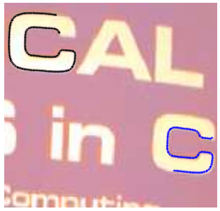
In the paper, the authors use the cover of a book that has two similar letter C's in the title. They detect the edges of the two C's as point clouds. The second C is then artificially rotated by some chosen angle which I will call the ground truth angle. The authors know the exact transformation to align the two C's on top of one another. They generate their 'basin of convergence' plot, by supplying different initial guesses for the rotation from the ground truth rotation minus 120 degress to plus 120 degrees. Therefore at 0 on their x axis, they are supplying the ground truth rotation to the solver.
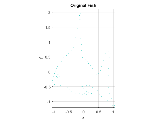
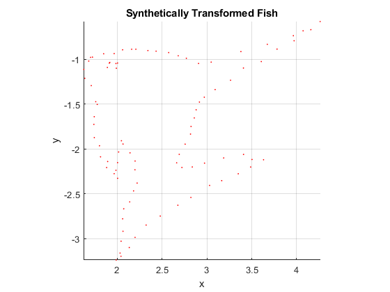
Since we do not have access to the original image used by the author, we use a 2D representation of a fish (shown below) and transform it by a 60 degree rotation and an arbitrary translation or 2.5 to the right and 1.75 below. We then add some gaussian noise to each transformed point to simulate the fact that the authors used two different letter C's that could have had some minor differences.
close all;
clear;
clc;

%Input
fish = load('fish.mat');
fish = fish.X;
icp_mins = [];
thetas = [];

% Ground Truth Transformation
ground_theta = 60;
t = deg2rad(ground_theta);
% Get 2D rotation matrix from rotation angle
r = [cos(t) sin(t); -sin(t) cos(t)];
t = [2.5; -1.75];
% Apply rotation to each point
transfish = (r*fish' + repmat(t,1,length(fish)))' + 0.01*randn(size(fish)) + 0.01;

% Here we represent the 2D pointcloud as a 3D point cloud since the ICP
% function we use for comparison takes 3D input
pfish = [fish(:,1) fish(:,2) zeros(length(fish),1 )];
ptransfish = [transfish(:,1) transfish(:,2) zeros(length(transfish),1 )];

pfish = pointCloud(pfish);
ptransfish = pointCloud(ptransfish, 'Color', [uint8(255.*ones(length(ptransfish),1)), zeros(length(ptransfish),1) zeros(length(ptransfish),1)]);


% Display the original and transformed pointcloud
figure(1);
pcshow(pfish, 'MarkerSize', 15);
title('Original Fish');
view([0 90]);
xlabel('x');
ylabel('y');
zlabel('z');

figure(2);
pcshow(ptransfish, 'MarkerSize', 15);
title('Synthetically Transformed Fish');
view([0 90]);
xlabel('x');
ylabel('y');
zlabel('z');
Proposed Solution
The proposed solution from the paper is to solve the step 2 minimization problem using the Levenberg Marquardt algorithm, which well suited to functions such as the one we have that are written in the form of a sum of squared residuals. The goal when using the algorithm is to find a new set of parameters, a(k + 1) given a(k) that reduces the error function. To do this, the vector of residual errors [e(a(k))] is computed using the equation in step 2. Correspondences of step 1 are found by selecting the closest point in the model for each data point. We can choose to set the weight of any point whose corresponding point is too far away to zero, but we found that our algorithm works well with keeping all the points. This makes sense because we have very little noise in the system.
After calculating the vector of residuals, the Jacobian (J) of this vector is calculated with respect to all the parameters. We will do this using finite backward differences.
The next step, and also the defining step of the Levenberg Marquardt algorithm is computing the update  so that
 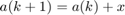 . The Levenberg Marquardt approach combines the Gauss Newton approach and the gradient descent approach while using
  to control whether to take small, safe, gradient descent steps or large, Gauss Newton steps.
We basically iterate these two steps until convergence.
Solution Implementation ICP
As mentioned before, we simply use Matlab's pcregrigid function. It finds the rigid transformation between two pointclouds using ICP algorithm. We study the minimum value of the objective function over an interval of [-120, 120] from the ground truth transformation. In the last figure of this report, the results over the entire interval are plotted along with the LM-ICP and LM-ICP-Huber method results.
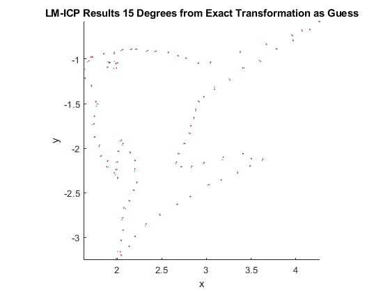
fun = @(a) double((vecnorm(transfish' - ([cos(a(1)) sin(a(1)); -sin(a(1)) cos(a(1))]*fish' + repmat([a(2) a(3)]',1,length(fish))))'));

for theta = ground_theta-120:1:ground_theta+120
    t = deg2rad(theta);
    r = [cos(t) sin(t); -sin(t) cos(t)];
    t = [2.5; -1.75];

    % pcregrigid function requires initial guess to be in the form of an
    % affine3d transformation. We are simply putting our 2D transformation
    % into that form.
    tform1 = affine3d([[r' [0 0]'; [0 0 1]], [0 0 0]'; [t' 0 1]]);
    inv_tform1 = invert(tform1);

    %Perform ICP using ground truth as initial guess
    [icp_tform, moving_reg, rmse] = pcregrigid(pfish, ptransfish, 'Extrapolate', true, 'InitialTransform', tform1);
    invr = invert(icp_tform);

    % Extract the parameter values from the returned solved transformation
    ak = icp_tform.T;
    solved_r = ak(1:2, 1:2);
    ak = [acos(solved_r(1,1)), ak(4,1), ak(4,2)];

    % The rms error of the Euclidean distance between the aligned point clouds
    e_ak = fun(ak);
    err = norm(e_ak)^2;

    icp_mins = [icp_mins; err];
    thetas = [thetas; theta-ground_theta];

    % Plot results for two specific cases. First case is where the initial
    % guess is the ground truth. Second is when the initial guess is 15
    % degrees from the ground truth.
    if (theta == ground_theta)
        %Display the overlap of transformed fish
        fish_icp_tform = pctransform(pfish, tform1);
        figure(3);
        hold on;
        pcshow(fish_icp_tform, 'MarkerSize', 15);
        pcshow(ptransfish, 'MarkerSize', 15);
        view([0 90]);
        title('ICP Results Exact Transformation As Guess');
        xlabel('x');
        ylabel('y');
        zlabel('z');
        hold off;
    elseif (theta == ground_theta+15)
        %Display the overlap of transformed fish
        fish_icp_tform = pctransform(pfish, tform1);
        figure(4);
        hold on;
        pcshow(fish_icp_tform, 'MarkerSize', 15);
        pcshow(ptransfish, 'MarkerSize', 15);
        view([0 90]);
        title('ICP Results 15 Degrees from Exact Transformation as Guess');
        xlabel('x');
        ylabel('y');
        zlabel('z');
        hold off;
    end

end
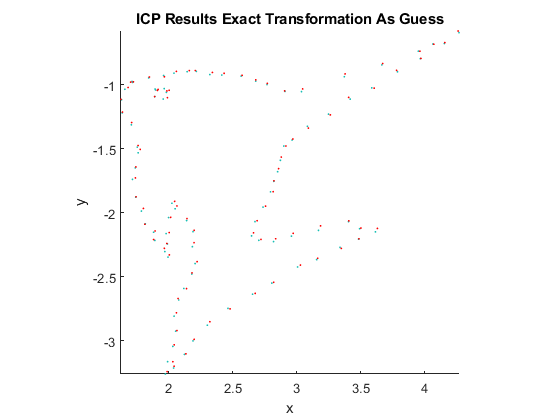
ICP Results Discussion
From the results, it can be seen that when the initial guess is the ground truth, the solver finds the correct transformation. As we get further away from the ground truth, the solver is still close to finding the correct transformation, but the solution is not exactly correct.
Solution Implementation LM-ICP and LM-ICP-Huber
This code is very similar to the above for the ICP implementation, except we use our function: lmicp_our instead of pcregrigid from Matlab. The function will be shown in the section below. We are again showing the results for two specific cases for each of the solutions for comparison.
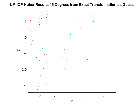
lm_mins = [];
lm_thetas = [];
lm_mins_huber = [];
lm_thetas_huber = [];

% Using standard Levenberg-Marquardt
for lm_theta = ground_theta-120:1:ground_theta+120
    a0 = [deg2rad(lm_theta) t'];
    [a, err] = lmicp_our(transfish, fish, a0, 0);

    lm_mins = [lm_mins; err];
    lm_thetas = [lm_thetas; lm_theta-ground_theta];

    if (lm_theta == ground_theta)
        %Display the overlap of transformed fish
        t = a(1);
        r = [cos(t) sin(t); -sin(t) cos(t)];
        t = a(2:3)';

        lm_transfish = (r*fish' + repmat(t,1,length(fish)))';

        lm_transfish = [lm_transfish(:,1) lm_transfish(:,2) zeros(length(lm_transfish),1 )];
        ptransfish = [transfish(:,1) transfish(:,2) zeros(length(transfish),1 )];

        lm_transfish = pointCloud(lm_transfish);
        ptransfish = pointCloud(ptransfish, 'Color', [uint8(255.*ones(length(ptransfish),1)), zeros(length(ptransfish),1) zeros(length(ptransfish),1)]);

        figure(5);
        hold on;
        pcshow(lm_transfish, 'MarkerSize', 15);
        pcshow(ptransfish, 'MarkerSize', 15);
        view([0 90]);
        title('LM-ICP Results Exact Transformation As Guess');
        xlabel('x');
        ylabel('y');
        zlabel('z');
        hold off;
    elseif (lm_theta == ground_theta+15)
        %Display the overlap of transformed fish
        t = a(1);
        r = [cos(t) sin(t); -sin(t) cos(t)];
        t = a(2:3)';

        lm_transfish = (r*fish' + repmat(t,1,length(fish)))';

        lm_transfish = [lm_transfish(:,1) lm_transfish(:,2) zeros(length(lm_transfish),1 )];
        ptransfish = [transfish(:,1) transfish(:,2) zeros(length(transfish),1 )];

        lm_transfish = pointCloud(lm_transfish);
        ptransfish = pointCloud(ptransfish, 'Color', [uint8(255.*ones(length(ptransfish),1)), zeros(length(ptransfish),1) zeros(length(ptransfish),1)]);

        figure(6);
        hold on;
        pcshow(lm_transfish, 'MarkerSize', 15);
        pcshow(ptransfish, 'MarkerSize', 15);
        view([0 90]);
        title('LM-ICP Results 15 Degrees from Exact Transformation as Guess');
        xlabel('x');
        ylabel('y');
        zlabel('z');
        hold off;
    end
end

for lm_theta = ground_theta-120:1:ground_theta+120
    a0 = [deg2rad(lm_theta) t'];
    [a, err] = lmicp_our(transfish, fish, a0, 1);

    lm_mins_huber = [lm_mins_huber; err];
    lm_thetas_huber = [lm_thetas_huber; lm_theta-ground_theta];

    if (lm_theta == ground_theta)
        %Display the overlap of transformed fish
        t = a(1);
        r = [cos(t) sin(t); -sin(t) cos(t)];
        t = a(2:3)';

        lm_transfish = (r*fish' + repmat(t,1,length(fish)))';

        lm_transfish = [lm_transfish(:,1) lm_transfish(:,2) zeros(length(lm_transfish),1 )];
        ptransfish = [transfish(:,1) transfish(:,2) zeros(length(transfish),1 )];

        lm_transfish = pointCloud(lm_transfish);
        ptransfish = pointCloud(ptransfish, 'Color', [uint8(255.*ones(length(ptransfish),1)), zeros(length(ptransfish),1) zeros(length(ptransfish),1)]);

        figure(7);
        hold on;
        pcshow(lm_transfish, 'MarkerSize', 15);
        pcshow(ptransfish, 'MarkerSize', 15);
        view([0 90]);
        title('LM-ICP-Huber Results Exact Transformation As Guess');
        xlabel('x');
        ylabel('y');
        zlabel('z');
        hold off;
    elseif (lm_theta == ground_theta+15)
        %Display the overlap of transformed fish
        t = a(1);
        r = [cos(t) sin(t); -sin(t) cos(t)];
        t = a(2:3)';

        lm_transfish = (r*fish' + repmat(t,1,length(fish)))';

        lm_transfish = [lm_transfish(:,1) lm_transfish(:,2) zeros(length(lm_transfish),1 )];
        ptransfish = [transfish(:,1) transfish(:,2) zeros(length(transfish),1 )];

        lm_transfish = pointCloud(lm_transfish);
        ptransfish = pointCloud(ptransfish, 'Color', [uint8(255.*ones(length(ptransfish),1)), zeros(length(ptransfish),1) zeros(length(ptransfish),1)]);

        figure(8);
        hold on;
        pcshow(lm_transfish, 'MarkerSize', 15);
        pcshow(ptransfish, 'MarkerSize', 15);
        view([0 90]);
        title('LM-ICP-Huber Results 15 Degrees from Exact Transformation as Guess');
        xlabel('x');
        ylabel('y');
        zlabel('z');
        hold off;
    end
end
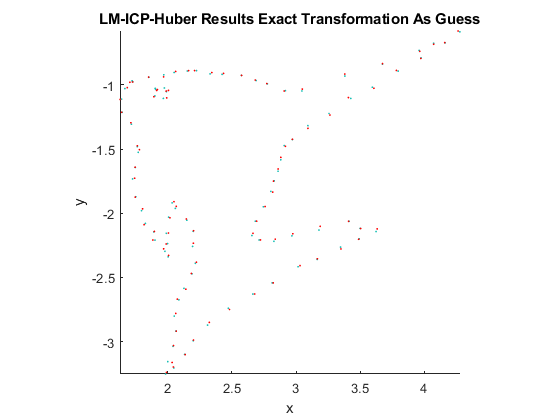
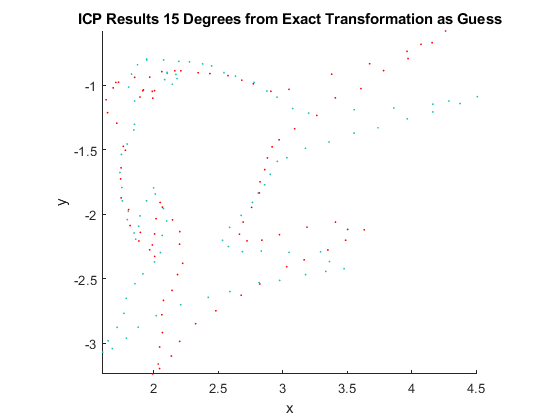
LM-ICP Results Discussion
From the results, it can be seen that our solver finds the correct transformation for both cases. In fact, we have visually verified that the solver finds the correct transformation for the basin showed at the end of this report.
LM-ICP Huber Results Discussion
From the results, it can be seen that when the initial guess is the ground truth, the solver finds the correct transformation. As we get further away from the ground truth, the solver is still close to finding the correct transformation, but the solution is not exactly correct. However, it still performs better than ICP. The basin for LM-ICP-Huber shown below is great for the entire interval. This means the minimum value of the objective function is always low for the solution found by LM-ICP with the Huber kernel. However, we notice that the solution is not correct. The algorithm has not converged to the correct global minimum. It is finding some local minimum.
The reason for this is that in our implementation, we did no take care to ensure that the LM algorithm behaves well if the kernel chosen is not smooth or if the derivatives of the objective function are smooth. We simply assumed that the derivatives behave smoothly and we calculate them using finite differencing. It is likely that the derivatives are in fact not smooth and we should account for this. Also, finite differencing only approximates the derivatives of the objective function and we may obtain different results if we use other methods or even use central difference instead of backwards difference as used in our implementation.
lmicp_our Function Implementation
We implemented our version of LM-ICP based on the information provided in the paper about the ICP and LM algorithms. The image below taken from the paper shows the LM algorithm they suggest.
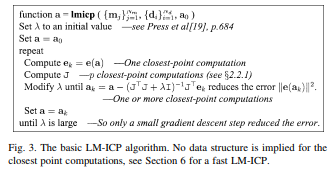
The main steps of our algorithm are as follows: Given our two point clouds (model and data) and an initial guess of parameters, we first calculate the correspondences of the points using the initial guess. To do this, we transform the data using the initial guess and take the closes point in the model as the correspondence for each data point. We then calculate the value of the objective function for these correspondences. Next, using the backward finite difference, we calculate the jacobian matrix of the objective function. That is to say that our calculation are of the form: 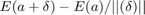 We also re calculate the correspondances for the new objective function while calculating the jacobian, as this is recommended by the authors. Finally, the next set of parameter values are calculate based on the Levenberg-Marquardt update rule:
  We continue to repeat these steps until our solution converges. The various convergence criteria used can be seen in the code below.
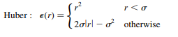
Adding the Huber kernal is straigtforward, based on the huber penalty function show in the paper (shown below). We simply allow our objective function througha huber kernel each time the objective function is calculated. Our function has a flag for when the huber kernel should be used.
function [a, currError] = lmicp_our(model, data, a0, huber)
    maxdist = 10000;
    thresh = 0.025; %0.0135;
    a = a0;

    % repeat step
    while (1)

        %transform the data using a0
        t = a(2:3)';
        r = [cos(a(1)) sin(a(1)); -sin(a(1)) cos(a(1))];
        transData = (r*data' + repmat(t,1,length(data)))';

        %find correspondences: take closest point as correspondence - multiple
        %points can be mapped to same point, closest points outside of distance
        %threshold maxdist are not mapped

        [k,d] = dsearchn(model, transData); %this matlab function does exactly what we need
        wi = double(d < maxdist);
        m = model(k, :);

        % preallocating matrices
        e_a = zeros(length(k), 1);
        J = zeros(length(k), length(a0));

        lambda = 0.001;
        theta = thresh.* ones(length(k), 1);

        while (lambda < 10^9) % One of the convergence criteria.. exit if lambda is large

            e_a = double(sqrt(wi).*(vecnorm(m' - ([cos(a(1)) sin(a(1)); -sin(a(1)) cos(a(1))]*data' + repmat([a(2) a(3)]',1,length(data))))'));

            if (huber)
                e_a = (((sqrt(e_a) < theta) .* (e_a)) + ((sqrt(e_a) >= theta) .* (2.*theta.*sqrt(e_a) - theta.^2)));
            end

            a_old = a;

            %Calculation of Jacobian based on backwards difference
            for j = 1:length(a0)
                da = 5e-3*ones(1, length(a0));
                da(j) = da(j)*(1 + abs(a(j)));
                a(j) = a(j) + da(j);

                %recalculate correspondences for more accurate solution
                t = a(2:3)';
                r = [cos(a(1)) sin(a(1)); -sin(a(1)) cos(a(1))];
                tD = (r*data' + repmat(t,1,length(data)))';
                [k,d] = dsearchn(model, tD);
                wi = double(d < maxdist);
                m = model(k, :);

                e_a1 = double(sqrt(wi).*(vecnorm(m' - ([cos(a(1)) sin(a(1)); -sin(a(1)) cos(a(1))]*data' + repmat([a(2) a(3)]',1,length(data))))'));

                if (huber)
                    e_a1 = (((sqrt(e_a1) < theta) .* (e_a1)) + ((sqrt(e_a1) >= theta) .* (2.*theta.*sqrt(e_a1) - theta.^2)));
                end

                J(:,j) = (e_a1 - e_a)/da(j);

                a = a_old;
            end

            % Calculate new set of parameters
            ak = a - ((J'*J + lambda*eye(length(a0)))\(J'*e_a))';

            % Calculate new objective function value
            e_ak = double(sqrt(wi).*(vecnorm(m' - ([cos(ak(1)) sin(ak(1)); -sin(ak(1)) cos(ak(1))]*data' + repmat([ak(2) ak(3)]',1,length(data))))'));

            if (huber)
                e_ak = (((sqrt(e_ak) < theta) .* (e_ak)) + ((sqrt(e_ak) >= theta) .* (2.*theta.*sqrt(e_ak) - theta.^2)));
            end

            prevError = norm(e_a);
            currError = norm(e_ak);

            if (currError >= prevError) % We are diverging... increase lambda
                lambda = lambda * 3;
            else % error is getting smaller
                lambda = lambda / 3;
                a = ak;
                if (prevError - currError < 1e-3) %If the error got smaller by a very small amount, we can stop
                    break;
                end
            end

        end

        if (a - ak < ones(1, length(a))*1e-3) % ICP convergence criteria, change in parameters is close to zero
            break;
        end

     end

end
Results
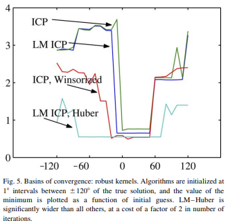
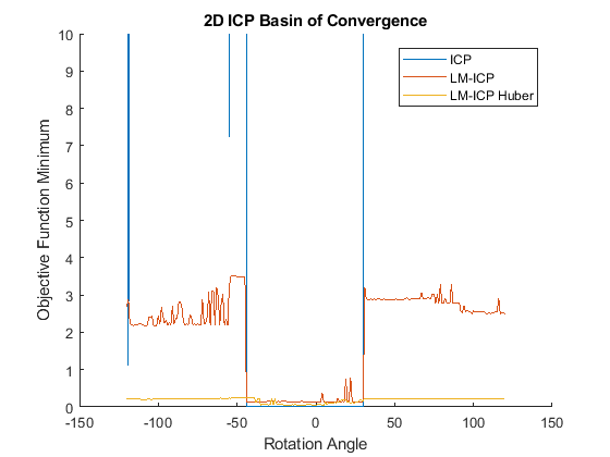
The basin of convergence graph that we generate based on our function is shown below. It can be seen that the graph is very similar to the one from the paper. The size of the basins for ICP and LM-ICP are similar and compare to the size of the paper's LM ICP. This is as expected since, Matlab's implementation of ICP is likely more optimized and better than the simple one used by the authors. It can be seen that our basin of convergence is more centered on the ground truth where as the authors basins for these two algorithms are more on the right side. We suspect this is due to the use of two different C shapes. Error is introduced also from the image processing algorithm used to detect the edges of the shapes. Our basin for the huber kernal spans the entire 240 degrees tested, whereas the author's basin is about half that size. We have realized that our Huber implementation has shortcomings due to the fact that we do not check to make sure our derivatives are always smooth. However, it was observed that the Huber kernel does a good job to bring the objective function value down by penalizing points that are far away. In this way, the solver is made robust.
figure(9)
hold on;
plot(thetas, icp_mins);
plot(lm_thetas, lm_mins);
plot(lm_thetas_huber, lm_mins_huber);
title('2D ICP Basin of Convergence');
xlabel('Rotation Angle');
ylabel('Objective Function Minimum');
legend('ICP', 'LM-ICP', 'LM-ICP Huber');
ylim([0 10])
Analysis and Conclusion
In conclusion, we were able to reproduce the results of the paper in the 2D case for the ICP and LM-ICP algorithms. Our implementation of the Huber LM-ICP was not on par with the papers and under performed. However, we know what we did wrong, and can agree that our own conclusions support those made by the authors. It is observed that the ICP problem can be solved via generalized optimization techniques which can help to robustify the solution as well.