Fast Maximum Margin Matrix Factorization for Collaborative Prediction
Research paper by Jason D. M. Rennie and Nathan Srebro [1], reproduced by ECE 602 students:
Omer Sheikh (20495239)
Filza Mazahir (20295951)
Dongwon Park (20700591)
Submiited on April 23, 2018
Contents
Problem formulation
Collaborative prediction in movie recommendations system takes as inputs user ratings on movies the users have already seen. Prediction of user preferences on movies they have not yet seen are then based on patterns in the partially observed rating matrix. This approach can be interpreted as that users "collaborate" by sharing their ratings, and can be formulated as a matrix completion problem—completing entries in a partially observed data matrix Y.
A common approach to collaborative prediction is to fit a factor model to the data, and use it to make further predictions. For  users and
  movies, we fit x target matrix
  with a
  matrix
  (a k-factor model). Then, the predictions are given by the product of an
  factor matrix
  and a
and a  coefficient matrix
  . Each row of U functions as a “feature vector” for each of the rows of . Each row of
  is a linear predictor, together with “features” in , predicting the entries in the corresponding column of . In 2005, Srebro et al. suggested a semi-definite programming (SDP) formulation (solvable using standard SDP solvers) of the collaborative prediction problem, named Maximum Margin Matrix Factorization (MMMF), by constraining the norms of and instead of their dimensionality [2]. However SDP solvers (at the time of the published paper) could only handle MMMF problems on matrices of dimensionality up to a few hundred (not realistically sized).
In this paper, the authors proposed a method for seeking a MMMF by directly optimizing the factorization  , that is, by using a gradient-based local serach technique on the matrics and . The method allows solving large (realistically sized) collaborative prediction problems.
Proposed solution
The problem can be formulated as a minimization problem of a dual objective function, where the objective function is the trace norm, combined with smooth hinge-loss. The solution of the problem, therefore, balances between low trace-norm and low error.
The trace norm  is a non-differentiable function for which it is not easy to find the subdifferential (Thus, finding good descent directions is not easy). With a factorization
  , for any
  we have
 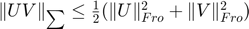 (
( denotes the Frobenius norm). Therefore, an unconstrained minimization problem is formulated as below:
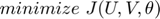
where:
 is smooth hinge loss function
 is a regularization constant
 is ordinal movie ratings
The smooth hinge loss, defined below, circumvents non-differentiability of the hinge loss function  at
at  :
:
Note that the MMMF objective function is a non-convex function. This can potentially inhibit convergence of the global minimum. However, the authors impirically showed that the solutions obtained from the above minimization problem are indeed very close to global optimums, and that local minima are, at worst, rare.
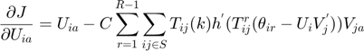
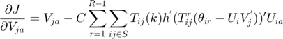
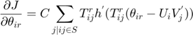
The partial derivatives of the MMMF objective function with respect to the optimization variables , and  are as follows:
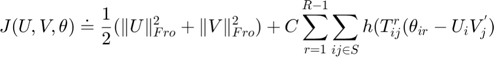
The real-valued  are related to the discrete movie ratings
 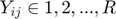 (e.g. 1–5 “stars”) by requiring
  where
where  thresholds
  are learned from the partially observed data matrix . The optimization algorithm searches over pairs of matrices
  , as well as sets of thresholds
  that together minimizes the objective function. With the continuous gradients in-hand, the authors used non-linear Conjugate Gradients (CG) algorithm, in particular, the Polak-Ribiére variant.
Data sources
The authors conducted experiments on the 1M Movielens dataset [3]. The dataset contains 1,000,209 anonymous ratings of approximately 3,900 movies made by 6,040 MovieLens users who joined MovieLens in 2000. For this project, we used 100k Movielens dataset [3]. Both datasets have an identical structure, with a difference in the number of ratings. Using a smaller dataset allowed us to train the model within a reasonable time, for the project submission.
The 100k Movielens dataset are of ordinal ratings  . The ratings are contained in the file "u.data" in the following format:
- UserIDs range between 1 and 943
- MovieIDs range between 1 and 1682
- 100,000 ratings (1-5) are made on a 5-star scale (whole-star ratings only)
- Timestamp is represented in seconds since since 1/1/1970 UTC (Neither the authors or we do not use Timestamp)
- Each user has at least 20 ratings
Below are some excerpts from the u.data file:
user id | item id | rating | timestamp
%196	242	3	881250949
%186	302	3	891717742
%22     377	1	878887116
%244	51	2	880606923
Data synthesis/import
The following code parses 100k MovieLens dataset into a partially observed data matrix , our training data. We also construct testing and validation matrices of zeros (or no ratings) with a size equivalent to . We randomly withheld two known movie ratings from each user and place them in the corresponding position of the testing and validation matrices (one for testing and one for validation), as was done in the paper [1]. The validation matrix is used for finding an optimal regularization constant (one with the lowest validation error among of a set of contants we supplied), and the testing matrix is used for assessing the accuracy of the output model.
global Y C R;
rng('default');
rng(325); % seed for reproducibility

% Running this code requires the MovieLens 100k dataset. See [3].
ratings = dlmread('./ml-100k/u.data', "\t");

n = 943;
m = 1682;
R = 5;
ml_data = zeros(n,m);
for i = 1:size(ratings, 1)
  user = ratings(i, 1);
  movie = ratings(i, 2);
  r = ratings(i, 3);
  ml_data(user, movie) = r;
end

% use 700 users for weak generalization
n = 700;
train = ml_data(1:n, :);
val = zeros(size(train));
test = zeros(size(train));

strong_train = ml_data(n+1:end, :);
strong_test = zeros(size(strong_train));

% To construct the testing and validation matrices, we remove 2 known
% values from every row in the "training" matrix and place one in the
% corresponding row in the validation matrix and similarly place one in the
% test matrix.
for i = 1:n
    idx = find(train(i, :));
    idx = idx(randperm(length(idx)));
    test(i, idx(1)) = train(i, idx(1));
    val(i, idx(2)) = train(i, idx(2));

    % hide the values being used for testing/validation
    train(i, idx(1)) = 0;
    train(i, idx(2)) = 0;
end

% Use remaining 243 users for strong generalization
for i = 1:size(strong_train, 1)
    idx = find(strong_train(i, :));
    idx = idx(randperm(length(idx)));
    strong_test(i, idx(1)) = strong_train(i, idx(1));
    strong_train(i, idx(1)) = 0;
end

clear ratings;
Numerical solution and demonstration
The MMMF objective function with smooth hinge-loss is not a convex function, making it difficult for us to use the CVX library. Matlab's solver for non-linear functions (fminunc) also was not apt for the problem at hand due to a large resulting Hessian matrix of size that exceeds the maximum array size. The authors used the Polak-Ribiére variant of CG algorithm (Shewchuk, 1994; Nocedal & Wright, 1999) with the consecutive gradient independence test (Nocedal & Wright, 1999) to determine when to “reset” the direction of exploration. They used the Secant line search suggested by (Shewchuk, 1994), which uses linear interpolation to find an approximate root of the directional derivative. Similarly, we implemented Polak-Ribiére variant of CG algorithm, but with backtracking line serach.
The dimensionality of and is unbounded because the norms of and are contrained instead of their dimensionality. Hence, a large rank  (the number of columns for and ) can be used. However, the authors showed that there is no need to consider rank larger than
  where and are the number of users (number of rows of
  ) and movies (number of columns of ), respectively. And, in practice, much smaller values of can be used. Using a small (hence, truncated , ) results in significantly faster learning than using . For experiments, the authors used
  ; we also used of 100 for results comparison purposes. The following code contains functions for:
- MMMF Objective function and its gradient (including smooth hinge function and its gradient)
- Polak-Ribiére non-linear CG algorithm with backtracking line search
- Normalized Mean absolute error function for results analysis
[n, m] = size(train);
k = 100;
x0 = randn(n*k + m*k + n*(R-1), 1);

Cs = [0.03, 0.1, 0.3, 1, 3];
Y = train;

best_error = Inf;
best_pred = Y;
best_C = 1;

for i = 1:length(Cs)
    tic;
    C = Cs(i);
    [x, fval, exititer] = prcg(x0, @mmmf, 10000, 1e-4);
    t = toc;
    [U, V, theta] = unpack_params(x, n, m, R);
    y_pred = predict(U, V, theta);
    train_error = nmae(train, y_pred);
    val_error = nmae(val, y_pred);
    fprintf('Weak Generalization: C = %f trained in %fs. Training NMAE = %f, Validation NMAE = %f\n', C, t, train_error, val_error);
    if val_error < best_error
        best_error = val_error;
        best_pred = y_pred;
        best_C = C;
        best_V = V;
    end
end
Weak Generalization: C = 0.030000 trained in 151.075042s. Training NMAE = 0.405567, Validation NMAE = 0.475893
Weak Generalization: C = 0.100000 trained in 172.262157s. Training NMAE = 0.069915, Validation NMAE = 0.453571
Weak Generalization: C = 0.300000 trained in 3721.534419s. Training NMAE = 0.001750, Validation NMAE = 0.470536
Weak Generalization: C = 3.000000 trained in 285.230398s. Training NMAE = 0.000108, Validation NMAE = 0.478571
test_error = nmae(test, best_pred);
fprintf('Best validation parameter C = %f\n', best_C);
fprintf('Best Weak Test NMAE = %f\n', test_error);
Best validation parameter C = 0.100000
Best Weak Test NMAE = 0.450893
Strong Generalization with remaining 243 users
[n, m] = size(strong_train);

% Feature matrices U and theta are user dependant.
U = randn(n, k);
theta = randn(n, R-1);
V = best_V; % use V trained by weak generalization
Y = strong_train;

x0 = [U(:); V(:); theta(:)];
[x, fval, exititer] = prcg(x0, @mmmf_V_frozen, 10000, 1e-4);
[U, V, theta] = unpack_params(x, n, m, R);
y_pred = predict(U, V, theta);
train_error = nmae(strong_train, y_pred);
test_error = nmae(strong_test, y_pred);

fprintf('Strong Train NMAE = %f, Test NMAE = %f\n', train_error, test_error);
Strong Train NMAE = 0.143174, Test NMAE = 0.550412
The authors illustrated that the objective decreases as k increases but above certain threshold of k, the objective value plateaus, for a given regularization constant, . Our analysis show a similar result.
Y = ml_data(1:100, :);
[n, m] = size(Y);
ks = [5, 10, 20, 30, 40, 50, 60, 70, 100];
objectives = zeros(size(ks));
C = best_C;
for i = 1:length(ks)
    tic;
    k = ks(i);
    x0 = randn(n*k + m*k + n*(R-1), 1);
    [x, fval, exititer] = prcg(x0, @mmmf, 10000, 1e-5);
    objectives(i) = fval;
    t = toc;
end

plot(ks, objectives);
ylabel('Objective');
xlabel('Rank of matrices U and V (k)');
The Objective Function.
% This function calculates the objective J(U, V, theta) and its associated gradient
% Expects x to be a vector in the shape [U(:), V(:), theta(:)]
% The returned gradient should then be in the same shape as x.
% Globals:
% Y the train set
% R the number of distinct rating values
% C the regularization scalar
function [J, dJ] = mmmf(x)
  global Y C R;
  [n, m] = size(Y);
  [U, V, theta] = unpack_params(x, n, m, R);

  trace_norm = (norm(U, 'fro')^2 + norm(V, 'fro')^2) / 2;
  X = U*V.';
  Yk_idx = Y > 0;
  Xk = Yk_idx .* X;

  loss = 0;
  dU = U;
  dV = V;
  dtheta = zeros(n, R-1);
  for r = 1:R-1
    % T_ij = -1 if r < Y_ij, 1 otherwise
    T = (Y > 0 & Y <= r) - (Y > r);
    theta_mat = repmat(theta(:, r), 1, m);
    Z = T .* (theta_mat  - Xk);
    loss = loss + sum(sum(smoothHinge(Z)));
    grad = T .* hingeGrad(Z);
    dV = dV - C * grad'*U;
    dU = dU - C * grad*V;
    dtheta(:, r) = C * grad*ones(m,1);
  end
  dJ = [dU(:); dV(:); dtheta(:)];
  J = trace_norm + C * loss;
end

% Matrix V is depends on the items. Leave it frozen for strong
% generalization
function [J, dJ] = mmmf_V_frozen(x)
  global Y C R;
  [n, m] = size(Y);
  [U, V, theta] = unpack_params(x, n, m, R);

  trace_norm = (norm(U, 'fro')^2 + norm(V, 'fro')^2) / 2;
  X = U*V.';
  Yk_idx = Y > 0;
  Xk = Yk_idx .* X;

  loss = 0;
  dU = U;
  dV = zeros(size(V)); % "freeze" V so that is not trained on
  dtheta = zeros(n, R-1);
  for r = 1:R-1
    % T_ij = -1 if r < Y_ij, 1 otherwise
    T = (Y > 0 & Y <= r) - (Y > r);
    theta_mat = repmat(theta(:, r), 1, m);
    Z = T .* (theta_mat  - Xk);
    loss = loss + sum(sum(smoothHinge(Z)));
    grad = T .* hingeGrad(Z);
    dU = dU - C * grad*V;
    dtheta(:, r) = C * grad*ones(m,1);
  end
  dJ = [dU(:); dV(:); dtheta(:)];
  J = trace_norm + C * loss;
end

% For making predictions after tuning U, V and theta
function y = predict(U, V, theta)
  X = U * V.';
  [n, m] = size(X);
  y = ones(n, m);
  [~, R_1] = size(theta);
  for i = 1:R_1
    y = y + (X >= repmat(theta(:,i), 1, m));
  end
end

% Helper function to unpack the param vector into U, V and theta.
function [U, V, theta] = unpack_params(x, n, m, R)
  theta = x(end - n*(R-1) + 1 : end);
  k = (length(x) - length(theta)) / (n+m);
  U = x(1:n*k);
  V = x(length(U) + 1 : length(U) + m*k);

  theta = reshape(theta, n, R-1);
  U = reshape(U, n, k);
  V = reshape(V, m, k);
end
Justification for using Conjugate Gradient Algorithm:
Using CVX was not viable as the objective function with smooth hinge loss was not convex. Using MATLAB's optimization toolbox was also unviable, the algorithms used by fminunc attempts to approximate the Hessian from the supplied gradient. Because of the size of the gradient vector (125140 for weak generalization), the Hessian is a 125140x125140 matrix, which is too large to store in memory. Algorithms in MATLAB's optimization toolbox that do not try to approximate the Hessian also do not utilize the objective gradient and thus are too slow to converge. Therefore, we wrote an impllementation Polak-Ribiére Conjugate Gradient algorithm [5] since this was the algorithm used the authors. However, we used a simpler backtracking line search based on the Armijo–Goldstein [4] condition.
% PR Conjugate Gradients Solver
function [x, J, exititer] = prcg(x0, func, maxiter, tol)
    i = 0;
    [J, dJ] = func(x0);

    dneg = -dJ;
    dneg_prev = dneg;
    d = dneg;

    x = x0;
    d2 = d'*d; % l2-norm squared
    d2_start = d2;
    while (i < maxiter) && (d2 > tol * d2_start)
        step = linesearch(func, d, x);
        x = x + step * d;

        [J, dJ] = func(x);
        dneg_prev = dneg;
        dneg = -dJ;
        beta = (dneg' * (dneg-dneg_prev)) / (dneg_prev'*dneg_prev);
        beta = max(0, beta);

        d = dneg + beta * d;
        d2 = d'*d;
        i = i + 1;
    end
    exititer = i;
end

% Backtracking line search
function [alpha] = linesearch(func, direction, x)
    c1 = 1e-4;
    delta = 0.5;
    alpha = 1;
    [J0, dJ0] = func(x);
    x0 = x;

    x = x0 + alpha * direction;
    [J, dJ] = func(x);
    while (J > J0 + c1 * alpha * (dJ0' * direction))
        alpha = delta * alpha;
        x = x0 + alpha * direction;
        [J, dJ] = func(x);
    end
end
The smooth hinge function and its gradient
function l = smoothHinge(z)
  % if z > 1 h(z) = 0
  % if z < 0, h(z) = 1/2 - z;
  low_z = z < 0;
  low_z = low_z .* (0.5 - z);

  % if z >= 0 and z < 1, h(z) = 1/2 - z + (z^2)/2
  hi_z = z >= 0 & z < 1;
  hi_z = hi_z .* (0.5 - z + (z.^2)./2);

  l = hi_z + low_z;
end

function d = hingeGrad(z)
  % z>1, grad = 0
  % z<0, grad = -1
  low_z = (z < 0) * -1;
  % 0<z<1, grad = z-1
  hi_z = (z >= 0 & z < 1);
  hi_z = (z - ones(size(z))) .* hi_z;
  d = low_z + hi_z;
end

function [error] = abs_error(y_true, y_pred)
    pred = (y_true > 0) .* y_pred;
    error = sum(sum(abs(y_true - pred)));
end

function [error] = mean_abs_error(y_true, y_pred)
    error = abs_error(y_true, y_pred) / sum(sum(y_true > 0));
end

% Nomalized mean absolute error, as described by Marlin (2004) for ratings=1..5
function [error] = nmae(y_true, y_pred)
    error = mean_abs_error(y_true, y_pred) / 1.6;
end
Visualization of results
“Weak generalization” is a single stage process which involves the learner filling-in missing entries of a rating matrix. “Strong generalization” is a two-stage process where the learner trains a model on one set of users and then is asked to make predictions on a new set of users. The learner is given sample ratings on the new set of users, but may not utilize those ratings until after the initial model is constructed [1]. The authors tested both types of generalization, “weak” and “strong.” Our Normalized Mean Absolute Error(NMAE) results are comparable but not as good as the results the authors obtained.
| Our Normalized Mean Absolute Error | Original Normalized Mean Absolute Error | |
|---|---|---|
| Weak Generalization | 0.4508 | 0.4156 |
| Strong Generalization | 0.5504 | 0.4203 |
In addition, we also verified the paper's claim that the rank of matrices U and V need not be too large. The objective function achieves similar values for k > 30 as shown in the plot in the previous section.
Analysis and conclusions
- Our results are reasonably close in terms of the NMAE to suggest that the optimization algorithm behaves in a predictable way.
- It has been shown that it is possible to “scale-up” MMMF to large problems by demonstrating the tecnique on the 1M MovieLens dataset (the authors) and on the 100k MovieLens dataset (us).
- The underlying assumption in a collaborative prediction situation is that the prediction tasks (columns of ) are related, in that the same features can be used for all of them, though possibly in different ways. This is proven to be a reasonably correct assumption based on the low NMAE (error magnitude).
- A downside of the proposed approach is that the objective function is not convex. This limits the optimization techniques that can be used and creates the possibility of converging to a local minimum instead of the global one.
References
[1] Rennie, J., Srebro, N., Fast maximum margin matrix factorization for collaborative prediction, in Proceedings of the International Conference of Machine Learning (2005)
[2] Srebro, N., Schraibman, A. Rank, trace-norm and max-norm. Proceedings of the 18th Annual Conference on Learning Theory.(2005).
[3] F. Maxwell Harper and Joseph A. Konstan. 2015. The MovieLens Datasets: History and Context. ACM Transactions on Interactive Intelligent Systems (TiiS) 5, 4, Article 19 (December 2015), 19 pages. DOI=http://dx.doi.org/10.1145/2827872
[4] L. Armijo. 1966. Minimization of functions having Lipschitz continuous first partial derivatives. Pacific J. Math. 16. no. 1, 1--3.
[5] J. R. Shewchuk. An Introduction to the Conjugate Gradient Method Without the Agonizing Pain. August 1994.