ECE 602 Project: Structured Sparsity through Convex Optimization
by Rui Zhou (20699091)and Jian Wang (20744992)
based on Structured Sparsity through Convex Optimization [1] and Structural Group Sparse Representation for Image Compressive Sensing Recovery [2].
Contents
- 1.Introduction
- 2.Problem Formulation
- 3.Proposed Solution
- - 3.1 Numerical Algorithm Implementation Details
- - 3.2 Adaptive Dictionary Learning
- - 3.3 Closed-form Solution for Structural Group Sub-problem
- - 3.4 Summary
- 4. Solution
- - 4.1 Construct Compressed Image
- - 4.2 Set Operation Conditions
- - 4.3 Implement IST Algorithms
- - 4.4 Reconstruct Structural Group
- - 4.5 Peak Signal-to-Noise Ratio
- 5. Analysis and Conclution
- References
1.Introduction
The structured sparsity is a natural extension of the standard sparsity concept in statistical learning and compressive sensing. It generalizes the group sparsity by allowing arbitrary structures on the feature set. Sparse estimation methods are aimed at using or obtaining parsimonious representation of data of models. With the development of research, the situations considered are not only about sparsity but also structural prior knowledge. A specific implementation explained in [1] and [2] is image restoration. Compressive Sensing (CS) solution space can be greatly confined by applying framework for image compressive sensing recovery via structural group sparse representation (SGSR) modeling.
2.Problem Formulation
The problem for CS recovery of a signal  said to be sparse in domain or basis
  from
from  is formulated as the following constrained optimization problem:
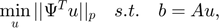
where  represents the random projections (RS).
The CS recovery using SGSR modeling is achieved by following steps. Firstly, the original image  is divided into several overlapped patches represented by
  . After that, for each patch in a given training window,
  best matched patches are searched, which consist of the set
  . Then, define the structural group
  corresponding to , which includes every element of as its columns. Finally, given the adaptive dictionary
  for each group
The CS recovery problem with the SGSR modeling now can be formulated as:
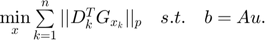
Set  to 0 for higher sparse representation. Let
  and
and  for the concentration of all
  . The CS problem shown above can be rewritten to:
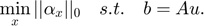
3.Proposed Solution
The optimization problem presented above is hard to solve due to the non-differentiability and non-linearity of the SGSR term.
- 3.1 Numerical Algorithm Implementation Details
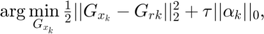
Add the regularization parameter and the problem can be transformed into the following unconstrained form:
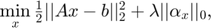
Then, invoking iterative shrinkage/thresholding algorithms (ISTA) leads to the following two iterative steps:


where  is a constant stepsize and
  denotes the iteration number. However, it is diffcult to solve the second step equation because of the complicated definition of .
Concretely,  can be regarded as some type of the noisy observation of , and then an assumption is made that each element of
  follows an independent zero-mean distribution with variance \sigma^{2}. There exists the following equation with very large probability (limited to 1):

With the help of the equation above, the problem is transfered to:
where  .
.
- 3.2 Adaptive Dictionary Learning
For each structural group , its adaptive dictionary is learned from its approximate estimate  .
.
Apply the singular value decomposition (SVD)to , we have:

where ![$\gamma_{k}=[\sigma_{r_{k}\otimes 1};\sigma_{r_{k}\otimes 2};...;\sigma_{r_{k}\otimes m}],$](./Project_main_files/Project_main_eq15089387259698020138.png)
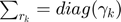 is a diagonal matrix with the elements of
  on its main diagonal, and
  are the columns of
  and
and  separately.
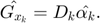
Define each atom  of adaptive dictionary for every group $G_{x_k}} as follows:

The learned adaptive dictionary is constructed by ![$D_{k} = [d_{{k} \otimes 1},d_{{k} \otimes 2},...,d_{{k} \otimes m}].$](./Project_main_files/Project_main_eq05567206247007512532.png)
- 3.3 Closed-form Solution for Structural Group Sub-problem
With the design of adaptive dictionary learning, we have the following result.

Thus, the sub_problem is equivalent to
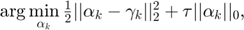
and the efficient solution for it is:
- 3.4 Summary
A rough summary of image CS recovery via SGSR is given below:
Input: The observed measurement  the measurement matrix and parameter
  ;
;
 Initialization: set initial estimate
  ;
;
for Iteration number = 0, 1, 2, ..., Max_iter
Update
Create structural groups by searching similar patches in new ;
for Each group
Construct dictionary ;
Reconstruct  ;
;
end for
Update by weighted averaging all the reconstructed groups ;
end for
Output: Final recovered image  .
.
4. Solution
- 4.1 Construct Compressed Image
% CS sampling rate
sample_rate = 0.2;

% Set block size
block_size = 32;

% The maximum number of iterations
max_iterations = 120;

% Constructe measurement matrix A (Gaussian Random)
N = block_size * block_size;
M = round(sample_rate * N);
randn('seed',0);
A = orth(randn(N, N))';
A = A(1:M, :);

% Load the original image  Vessels96.tif
image_name = 'Vessels96.tif';
original_image = double(imread(image_name));

[row, col] = size(original_image);

x = im2col(original_image, [block_size block_size], 'distinct');

% Get compressed signal
b = A * x;
- 4.2 Set Operation Conditions
The method to calculate initial x is introduced in [3] and the function MH_BCS_SPL Decoder comes from [4].
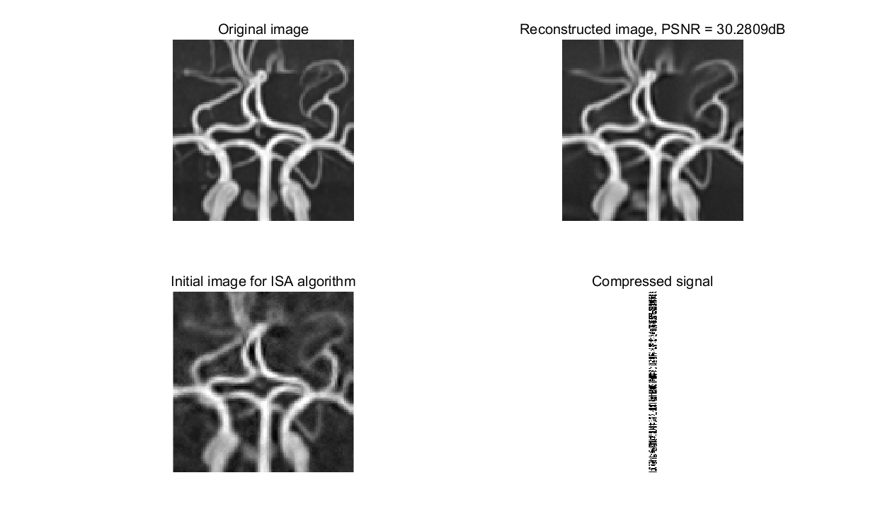
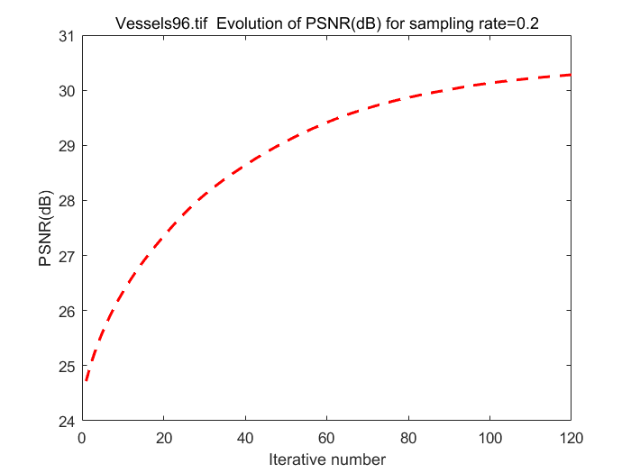
% Obtain Initial x
[~, x_initial] = MH_BCS_SPL_Decoder(b, A, sample_rate, row, col);

Opt_cond = [];
Opt_cond.A = A;
Opt_cond.block_size = block_size;
Opt_cond.org = original_image;
Opt_cond.max_iterations = max_iterations;
Opt_cond.row = row;
Opt_cond.col = col;
Opt_cond.initial = double(x_initial);
Opt_cond.lambda = 9.4;

% Invoke Proposed SGSR Alogorithm for Block-based CS Recovery
[reconstructed_image, psnr_all]= ISTA(b, Opt_cond);

% Get final PSNR for quality estimation
psnr = PSNR(original_image, reconstructed_image, 2);

% Print results
figure(1)
h=figure(1);
subplot(2,2,1);
imshow(uint8(original_image));
title('Original image', 'FontSize',12);

subplot(2,2,2);
imshow(uint8(reconstructed_image));
title (['Reconstructed image, PSNR = ',num2str(psnr), 'dB'],'FontSize',12);

subplot(2,2,3);
imshow(uint8(x_initial));
title ('Initial image for ISA algorithm','FontSize',12);

subplot(2,2,4);
imshow(b);
title ('Compressed signal','FontSize',12);
set (h,'position',[100 100 1000 600]);

figure(2)
plot (1:Opt_cond.max_iterations, psnr_all,'r--', 'LineWidth',1.8);
title (strcat(image_name,'  Evolution of PSNR(dB) for sampling rate=0.2'));
xlabel ('Iterative number');
ylabel ('PSNR(dB)');

snapnow
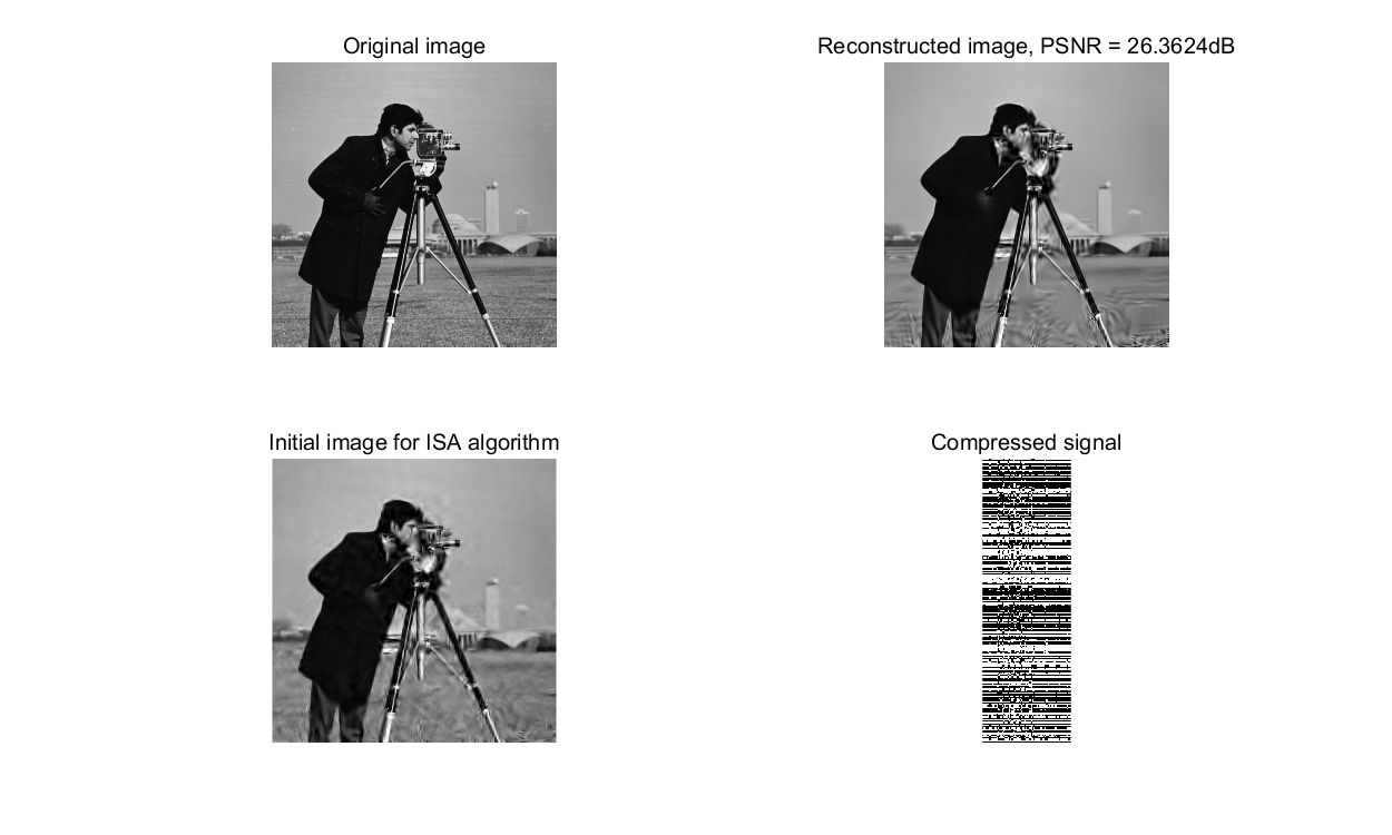
The following part is just the same as previous two sections while a larger image is operated for comparsion.
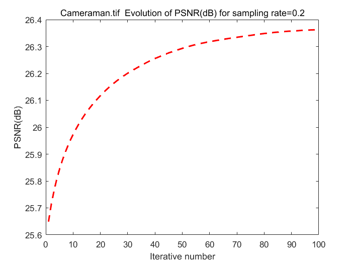
image_name = 'Cameraman.tif';
max_iterations = 100;

original_image = double(imread(image_name));

[row, col] = size(original_image);
x = im2col(original_image, [block_size block_size], 'distinct');

% Get compressed signal
b = A * x;

% Obtain Initial x
[~, x_initial] = MH_BCS_SPL_Decoder(b, A, sample_rate, row, col);

Opt_cond.org = original_image;
Opt_cond.max_iterations = max_iterations;
Opt_cond.row = row;
Opt_cond.col = col;
Opt_cond.initial = double(x_initial);

% Invoke Proposed SGSR Alogorithm for Block-based CS Recovery
[reconstructed_image, psnr_all]= ISTA(b, Opt_cond);

% Get final PSNR for quality estimation
psnr = PSNR(original_image, reconstructed_image, 2);

% Print results
figure(3)
g=figure(3);
subplot(2,2,1);
imshow(uint8(original_image));
title('Original image', 'FontSize',12);

subplot(2,2,2);
imshow(uint8(reconstructed_image));
title (['Reconstructed image, PSNR = ',num2str(psnr), 'dB'],'FontSize',12);

subplot(2,2,3);
imshow(uint8(x_initial));
title ('Initial image for ISA algorithm','FontSize',12);

subplot(2,2,4);
imshow(b);
title ('Compressed signal','FontSize',12);
set (g,'position',[100 100 1000 600]);

figure(4)
plot (1:Opt_cond.max_iterations, psnr_all,'r--', 'LineWidth',1.8);
title (strcat(image_name,'  Evolution of PSNR(dB) for sampling rate=0.2'));
xlabel ('Iterative number');
ylabel ('PSNR(dB)');

snapnow
- 4.3 Implement IST Algorithms
This is the part to implement ISA algorithms mentioned in section 3.1. The constant stepsize is set to 1 here.
function [reconstructed_image, psnr_all] = ISTA(b, Opt_cond)

row = Opt_cond.row;
col = Opt_cond.col;
A = Opt_cond.A;
x_org = Opt_cond.org;
max_iterations = Opt_cond.max_iterations;
x_initial = Opt_cond.initial;
block_size = Opt_cond.block_size;

x = im2col(x_initial, [block_size block_size], 'distinct');

% Store all PSNR values with the change of iterations
psnr_all = zeros (1,max_iterations);

for i = 1:1:max_iterations
    r = col2im(x, [block_size block_size],[row col], 'distinct');
    % r1 is x_j+1 and this is the step 2 in ISA algorithm
    % The SGSR function is used to solve sub-problem mentioned in
    % section 3.2
    r1 = SGSR(r, Opt_cond);
    r1 = im2col(r1, [block_size block_size], 'distinct');

    % x is r_j and this is the step 1 in ISA algorithm
    x = r1 - A'*A * r1 + A'*b;

    x_img = col2im(x, [block_size block_size],[row col], 'distinct');

    % Calculate PSNR in current iteration
    psnr_current = PSNR(x_img, x_org, 1);
    psnr_all(i) = psnr_current;
end
% obtain reconstructed image
reconstructed_image = col2im(x, [block_size block_size],[row col], 'distict');
end
- 4.4 Reconstruct Structural Group
This is actually the procedure to obtain solution of sub-problem in section 3.2. The recovered image can be represented using the average of all structural groups.

where  represents division for corresponding elements between two vectors and
  is a
is a  matrix with all elements are 1.
function [x_bar] = SGSR(r, Opt_cond)

% Set the size of overlapped patches from image
patch_size = 8;
patch_size_2D = patch_size * patch_size;

% Set the sliding distance of training window
sliding_distance = 4;

% Set the factor k/N
factor = 240;

% Set the number of best matched patches to be searched
number = 50;

% Set the size of training window
search_window = 10;

[L, W] =  size(r);
image_temp = zeros(L, W);
image_weight = zeros(L, W);

tau = Opt_cond.lambda * factor;
threshold = sqrt(2 * tau);

n  =  L - patch_size + 1;
m  =  W - patch_size + 1;
S  =  n * m;

% S_k
patch_set  =  zeros(patch_size_2D, S, 'single');

row  =  (1:sliding_distance:n);
row  =  [row row(end)+1:n];
column  =  (1:sliding_distance:m);
column  =  [column column(end)+1:m];

count = 0;
for i  = 1:patch_size
    for j  = 1:patch_size
        count  =  count + 1;
        patch  =  r(i:L - patch_size + i,j:W - patch_size + j);
        patch  =  patch(:);
        patch_set(count,:) =  patch';
    end
end

patch_set_T = patch_set';

I = (1:S);
I = reshape(I, n, m);
l_n = length(row);
l_m =  length(column);

patch_array = zeros(patch_size, patch_size, number);

for  i = 1:l_n
    for  j = 1:l_m
        row_current = row(i);
        column_current = column(j);
        off = (column_current - 1) * n + row_current;

        patch_index  =  Search(patch_set_T, row_current, column_current, off, number, search_window, I);
        current_array = patch_set(:, patch_index);

        % Singular value decomposition
        [Sg_s, Sg_v, Sg_d] = svd(current_array);

        % Hard threshold
        Sg_z = Sg_v.*(abs(Sg_v)>threshold);
        current_array = Sg_s * Sg_z * Sg_d';

        for k = 1:number
            patch_array(:,:,k) = reshape(current_array(:,k),patch_size,patch_size);
        end

        for k = 1:length(patch_index)
            % Compute row number
            if mod(patch_index(k), n) == 0
                row_index = n;
            else
                row_index = mod(patch_index(k),n);
            end

            % Compute column number
            col_index  =  ceil(double(patch_index(k))/ n);

            image_temp(row_index:row_index+patch_size-1, col_index:col_index+patch_size-1) = image_temp(row_index:row_index+patch_size-1, col_index:col_index+patch_size-1) + patch_array(:,:,k)';
            image_weight(row_index:row_index+patch_size-1, col_index:col_index+patch_size-1) = image_weight(row_index:row_index+patch_size-1, col_index:col_index+patch_size-1) + 1;
        end
    end
end

% Obtain the recovered image
x_bar = image_temp./(image_weight + eps);
return;
end
The following function aims to search best matched patches for each patch in the  training window and the measurement used to calculate similarity of patches is Euclidean distance.
function  index  =  Search(patch_set_T, row_current, column_current, off, number, search_window, I)

[n, m] = size(I);
dim = size(patch_set_T,2);

rmin = max( row_current - search_window, 1 );
rmax = min( row_current + search_window, n );
cmin = max( column_current - search_window, 1 );
cmax = min( column_current + search_window, m );

idx = I(rmin:rmax, cmin:cmax);
idx = idx(:);
a = patch_set_T(idx, :);
b = patch_set_T(off, :);

distance = (a(:,1) - b(1)).^2;

for k = 2:dim
    distance = distance + (a(:,k) - b(k)).^2;
end
distance = distance./dim;

[~, ind] = sort(distance);

index = idx( ind(1:number) );
end
- 4.5 Peak Signal-to-Noise Ratio
The peak signal-to-noise ratio (PSNR) is an engineering term for the ratio between the maximum possible power of a signal and the power of corrupting noise that affects the fidelity of its representation.
The PSNR(in dB) is defined as:
where  is the maximum possible pixel value of the image and
  is the mean square error between image and noisy approximation. The code for it using in this project is shown below.
function r = PSNR(I, K, flag)
    % For the pixels are represented using 8 bits per sample, MAX is 255.
    switch flag
        case 1
            I = double(I);
            K = double(K);
            error = I - K;

            [a, b, c] = size(I);

            if c ==1
                error = error(1:a,1:b);
                r = 10 * log10(255^2/mean(mean(error.^2)));
            else
                error=error(1:a,col+1:b,:);
                e1=error(:,:,1); e2=error(:,:,2);e3=error(:,:,3);
                r(1)= 10 * log10(255^2/mean(mean(e1.^2)));
                r(2)= 10 * log10(255^2/mean(mean(e2.^2)));
                r(3)= 10 * log10(255^2/mean(mean(e3.^2)));
            end
        case 2
            error = I - K;
            r = 10 * log10(255^2 / mean(error(:).^2));
    end
end
5. Analysis and Conclution
The PSNR for final reconstructed image is slightly lower than the result presented in the paper. There are mainly three reasons cause this difference and can be improved in further works.
1. The size of image affects the running time of program significantly so some operation conditions such as the size of patch and training window are expected to be adaptively changed.
2. The initial x selected in the IST algorithm can affect result significantly.
3. The values of some parameters such as the factor k/N and penalty parameter selected in operations can also affect result.
The image sparsity and self-similarity are enforced under a unified framework in an adaptive group dpmain by SGSR medeling. The IST algorithm presented in the paper to solve SGSR model based l0-norm optimizatino problem shows high performance in CS image recovery which is demonstrated in this project. However, the algorithm still needs to be improved for large image since the iteration is pretty slow in that case.
References
[1] F. Bach, R. Jenatton, J. Mairal and G. Obozinski."Structured Sparsity through Convex Optimization." Statistical Science, vol. 27, no. 4, pp. 450-468, 2012.
[2] J. Zhang, D. Zhao, F. Jiang and W. Gao. "Structural Group Sparse Representation for Image Compressive Sensing Recovery." 2013 Data Compression Conference.
[3] C. Chen, E. W. Tramel and J. E. Fowler. "Compressed-Sensing Recovery of Images and Video Using Multihypothesis Predictions." 45th Asilomar Conference on signals, Systems, and Computers.
[4] BCS-SPL package and MH-BCS-SPL Package (http://www.ece.msstate.edu/~fowler/BCSSPL/)