ECE 602 Course Project: Throughput Maximization in Wireless Powered Communication Networks
Team member: Huaqing Wu (20704063), Haixia Peng (20535999)
Contents
Problem formulation
A “harvest-then-transmit” protocol is proposed for wireless powered communication networks (WPCNs), where all users first harvest the wireless energy broadcast by the hybrid access point (H-AP) in the downlink (DL) and then send their independent information to the H-AP in the uplink (UL) by time-division-multiple-access (TDMA). Authors were interested in maximizing the UL throughput of by optimally allocating the time for the DL wireless energy transfer (WET) by the H-AP and the UL wireless information transmissions (WITs) by different users. With the proposed protocol, the authors first maximize the sum-throughput of the WPCN (referred to as sum-throughput maximization problem) by jointly optimizing the time allocated to the DL WET and the UL WITs given a total time constraint, based on the users' DL and UL channels as well as their average harvested energy amount. However, the sum-sumthroughput maximization solution is shown to allocate substantially more time to the near users than the far users, thus resulting in unfair achievable rates among different users, reffered to as “doubly near-far” phenomenon. To overcome this phenomenon, by proposing a new performance metric referred to as common-throughput with the additional constraint that all users should be allocated with an equal rate in their UL WITs regardless of their distances to the H-AP, a common-throughput maximization problem is formulated.
The sum-throughput maximization problem is formulated as
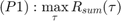


where,  is the number of users,
  represent the time portions in each block allocated to the H-AP (
 ) and users
  ,
,  is the sum-throughput of all users and given by
 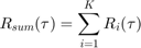 .
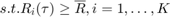
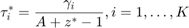
.  is the achievable UL throughput of user
  in bits/second/Hz (bps/Hz), and can be expressed as
 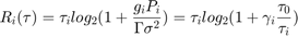 , where
  denotes the average transmit power at ,
  is the channel power gains of the reversed UL channel to user ,
  represents the signal-to-noise ratio (SNR) gap from the additive white Gaussian noise (AWGN) channel capacity due to a practical modulation and coding scheme (MCS) used,
  . In which,
  denotes the transmit power at the H-AP,
  is the channel power gains of the DL channel from the H-AP to user , and
  is the energy harvesting efficiency at each receiver (it is assumed to be same for each receiver).
The common-throughput maximization problem is formulated as


where,  denotes the common-throughput and
  is the feasible set of
  specified by
  and
and 
 .
.
Figure 3 in the paper shows the throughput given in (P1) for the special case of one single user in the network, i.e., K = 1, versus the time allocated to the DL WET,  , with
  , assuming that holds with equality, i.e., for the UL WIT
  .
.
gamma1 = 10;
tau0 = 0 : 0.001 : 1;
R = zeros(1,length(tau0)); R_max = 0;
for i = 1:length(tau0)
    R(i) = (1-tau0(i))*log2(1 + gamma1*tau0(i)/(1-tau0(i)));
    if R(i) > R_max
        R_max = R(i);
        tau_opt = tau0(i);
    end
end
figure;
plot(tau0,R,'b-','linewidth',2)
grid on;
xlabel('\tau_0','fontsize',12);
ylabel('Throughput (bps/Hz)','fontsize',12);
title('Fig. 3 in the Paper');
disp(['the optimal value of tau_0 is:', num2str(tau_opt)])
the optimal value of tau_0 is:0.418

Observing the figure, we can find that there exist an optimal value of , which means that the time allocated to the DL wireless energy transfer should not be too large or too small.
Solution for Problem P1
For the sum-throughput maximization problem (P1), since is a concave function of for any given  , which follows that is also a concave function of since it is the summation of 's. Therefore, (P1) is a convex optimization problem, and thus can be solved by convex optimization techniques. On the other hand, lemma 3.2 is defined as: given
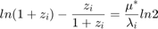
  , there exists a unique
  that is the solution of
  , where
  ,
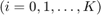
,  . Fig.4 shows that f(z) is a convex function over
  where the minimum is attained at
  with
with  . Therefore, given
  , there are two different solutions for , among which one is smaller than
  and the other is larger than , i.e., . On the other hand, if
  , there is only one solution for
  , which is larger than , i.e., .
z = 0 : 0.001 : 5;
f = z.*log(z) - z +1;
figure;
plot(z,f,'b-','linewidth',2)
grid on;
xlabel('z','fontsize',12);
ylabel('f(z)','fontsize',12);
title('Fig. 4 in the Paper');
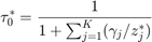
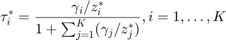
Thus, based on Proposition 3.1 in the paper, the optimal time allocation solution for (P1), denoted by ![$$\tau^\ast=[\tau_0^\ast \ \tau_1^\ast \ \ldots \ \tau_K^\ast]$](./main_files/main_eq00479341013337586725.png) , is given by
, is given by
 ,
,
where  and is the corresponding solution of f (z) = A as given by Lemma 3.2.
The optimal time allocation solution for (P1) follows that 
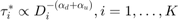 , which results in an unfair time and throughput allocation among users in the WPCN, i.e., the "doubly near-far" phenomenon. Here,
  and
and  denote the channel pathloss exponents in the DL and UL,respectively, and
  denotes the distance between the H-AP and . Fig.5 is used to further illustrate the "doubly near-far" phenomenon.
K = 2;
gamma_dB = [22, 10]; % the values of gamma in dB
gamma = 10.^(gamma_dB ./ 10);

% plot Fig 5 in the paper
tau_temp = 0.001:0.001:1;
[tau_1,tau_2] = meshgrid(0.001:0.001:1);
N_5 = length(tau_1);
R1_5= zeros(size(tau_1));
R2_5 = zeros(size(tau_1));
R_sum_5 = zeros(size(tau_1));
for i = 1 : N_5
    for j = 1 : N_5
        if tau_1(i,j) + tau_2(i,j) < 1
            R1_5(i,j) = tau_1(i,j)*log2(1+gamma(1)*(1-tau_1(i,j)-tau_2(i,j))/tau_1(i,j));
            R2_5(i,j) = tau_2(i,j)*log2(1+gamma(2)*(1-tau_1(i,j)-tau_2(i,j))/tau_2(i,j));
            R_sum_5(i,j) = R1_5(i,j) + R2_5(i,j);
        end
    end
end
figure;
contour(tau_1,tau_2,R_sum_5,10);
hold on
grid on;
xlabel('\tau_1 (allocated to U_1)','fontsize',12);
ylabel('\tau_2 (allocated to U_2)','fontsize',12);
title('Fig. 5 in the Paper');

% find the maximum value of the throughput and the corresponding tau
[m,n] = find(R_sum_5 == max(max(R_sum_5)));
tau_opt = [tau_1(m,n), tau_2(m,n)];
R1_opt_5 = R1_5(m,n);
R2_opt_5 = R2_5(m,n);
plot(tau_opt(1), tau_opt(2),'*')
disp(['the optimal value of tau is: [tau_0, tau_1, tau_2] = ', num2str([1-sum(tau_opt), tau_opt])])

% when calculating tau by proposition 3.1
tau_opt_5 = Optimal_tau_func_pro3(K, gamma);
disp(['the optimal value of tau based on Proposition 3.1 is: [tau_0, tau_1, tau_2] = ', num2str([tau_opt_5])])
the optimal value of tau is: [tau_0, tau_1, tau_2] = 0.244       0.711       0.045
the optimal value of tau based on Proposition 3.1 is: [tau_0, tau_1, tau_2] = 0.24447     0.71068    0.044841
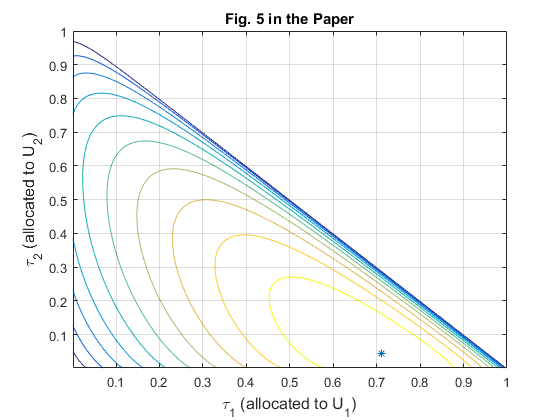
Fig.5 shows the sum-throughput versus UL WIT time allocation  and
and  for a two-user network with
  and
and  . It is assumed that the channel reciprocity holds for the DL and UL and thus
  , with
  , and
, and  ,
,  , with
 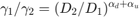 . We can also see from the results that, the optimal solution found by brute force is the same as that obtained by using Proposition 3.1, which validates the correctness of the proposition.
With the same setup as for Fig. 5, Fig. 6 shows the optimal throughput of  ,
,  , normalized by that of
  ,
,  , in a WPCN versus that in a conventional TDMA network for different values of the pathloss exponent
  , with
  . For the WPCN,
  is set to be fixed as for , while
  ,and
,and  for
for 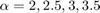 , and
, and  , respectively, since
  . For the conventional TDMA network,
  for both and are assumed to be
  with
with  and
and  denoting the average harvested energy at and in the WPCN under comparison, respectively; it then follows that for the conventional TDMA network,
  for , and
  ,and
,and  for , and , respectively.
alpha = 2 : 0.5 : 4;
N = length(alpha);

% For WPCN, the values of gamma are set as follows according to the paper
gamma1_wpcn = 10^(2.2);
gamma2_wpcn = [10^(1), 10^(0.7), 10^(0.4), 10^(0.1), 10^(-0.2)];
R2_R1_wpcn = zeros(1, N);
for i = 1 : N
    gamma_w = [gamma1_wpcn,gamma2_wpcn(i)];
    tau_opt_w = Optimal_tau_func_pro3(K, gamma_w);
    R1 =  tau_opt_w(2) * log2(1 + gamma_w(1)*tau_opt_w(1) / tau_opt_w(2));
    R2 =  tau_opt_w(3) * log2(1 + gamma_w(2)*tau_opt_w(1) / tau_opt_w(3));
    R2_R1_wpcn(i) = R2 / R1;
end

% For conventional TDMA network
gamma1_t = 10^(1.3);
gamma2_t = [10^(0.71) 10^(0.55) 10^(0.4) 10^(0.24) 10^(0.09)];
R2_R1_tdma = zeros(1, N);
for i = 1 : N
    gamma_t = [gamma1_t,gamma2_t(i)];
    tau_opt_t = Optimal_tau_func_pro3(K, gamma_t);
    R1 =  tau_opt_t(2) * log2(1 + gamma_t(1)*tau_opt_t(1) / tau_opt_t(2));
    R2 =  tau_opt_t(3) * log2(1 + gamma_t(2)*tau_opt_t(1) / tau_opt_t(3));
    R2_R1_tdma(i) = R2 / R1;
end
% plot Fig 6 in the paper
figure
semilogy(alpha,R2_R1_tdma, 'r-o ', alpha,R2_R1_wpcn, 'b-d ', 'linewidth',2)
xlabel('Pathloss Exponent, \alpha_d = \alpha_u = \alpha','fontsize',12);
ylabel('R_2 (\tau^*) / R_1 (\tau^*)','fontsize',12);
legend('Conventional TDMA network','WPCN');
grid on
title('Fig. 6 in the Paper');
Solution for Problem P2
To solve (P2), given any  , the following feasiblity problem is first considered,


Since the problem in (12) is convex, the authors consider its Lagrangian given by
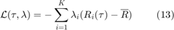
where ![$$\lambda = [\lambda_1,\ldots, \lambda_K] \succeq 0$](./main_files/main_eq14699766070415482662.png) consists of the Lagrange multipliers associated with the K user throughput constraints in problem (12). The dual function of problem (12) is then given by
consists of the Lagrange multipliers associated with the K user throughput constraints in problem (12). The dual function of problem (12) is then given by
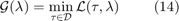
The dual function  can be used to determine whether problem (12) is feasible, as provided in lemma 4.1: For a given
  , problem (12) is infeasible if and only if there exists an
  such that
  .
.
Thus, in (14) can be obtained for a given by solving the following weighted sum-throughput maximization problem, which follows from (13).
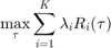
The problem in (15) is convex and thus can be solved by convex optimization techniques. Therefore, for the sum-throughput maximization case with  , the optimal time allocation solution for the weighted sum-throughput maximization problem in (15) is given as following proposition.
Proposition 4.1: Given , the optimal time allocation solution for (15), denoted by ![$$\tau^\ast=[\tau_0^\ast \tau_1^\ast \ldots \tau_K^\ast]$](./main_files/main_eq03782103061981180856.png) , is
, is
 ,
,
where  ,
,  , is the solution of the following equations:
 ,
,
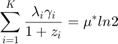 ,
,
with  being a constant.
Based on the above analysis, one iterative optimization algorithm to solve (P2) is given as follows,
1) Initialize  ,
, 
2) Repeat
 .
.- Initialize .
- Given
 , solve the problem in (15) by Proposition 4.1.
 - Compute using (13).
- If
 , is infeasible, set
  , go to step 1. Otherwise, update using sub-gradient based algorithms (e.g., the ellipsoid method) and the subgradient of given by (20). If the stopping criteria of the sub-gradient based algorithm is not met, go to step 3.
 - Set
 .
.
3) Until  , where
  is a given error tolerance.
where ![$$\nu ={[\nu_1 \nu_2 \ldots \nu_K]}^T$](./main_files/main_eq03729093240541116418.png) is the subgradient of .
is the subgradient of .
Fig. 7 shows the common-throughput in bps/Hz versus and for the same two-user channel setup as for Fig. 5.
[tau_1,tau_2] = meshgrid(0.001:0.001:1);
R_aver = zeros(size(tau_1));
for i = 1:length(tau_1)
    for j = 1:length(tau_1)
        if tau_1(i,j) + tau_2(i,j) < 1
            R1 = tau_1(i,j) * log2(1 + gamma(1)*(1-tau_1(i,j)-tau_2(i,j)) / tau_1(i,j));
            R2 = tau_2(i,j) * log2(1 + gamma(2)*(1-tau_1(i,j)-tau_2(i,j)) / tau_2(i,j));
            R_aver(i,j) = min(R1, R2);
        end
    end
end
figure
contour(tau_1,tau_2,R_aver,10);
hold on
grid on;
xlabel('\tau_1 (allocated to U_1)','fontsize',12);
ylabel('\tau_2 (allocated to U_2)','fontsize',12);
title('Fig. 7 in the Paper')

% find the optimal value of tau
[m,n] = find(R_aver == max(max(R_aver)));
tau_opt = [tau_1(m,n), tau_2(m,n)];
plot(tau_opt(1), tau_opt(2),'*')

% calculate the corresponding R(tau)
R1_opt_7 = tau_opt(1) * log2(1 + gamma(1)*(1-sum(tau_opt)) / tau_opt(1));
R2_opt_7 = tau_opt(2) * log2(1 + gamma(2)*(1-sum(tau_opt)) / tau_opt(2));
disp(['the optimal value of tau is: [tau_0, tau_1, tau_2] = ', num2str([1-sum(tau_opt), tau_opt])])
disp(['the optimal values of R1 and R2 are: [R1, R2] = ', num2str([R1_opt_7, R2_opt_7])])
disp(['the optimal common throughput is: min(R1, R2) = ', num2str(min(R1_opt_7, R2_opt_7))])
% calculate the throughput based on the optimal tau given in the paper
tau_given = [0.3683, 0.1386, 0.4932];
R1 = tau_given(2) * log2(1 + gamma(1)*tau_given(1) / tau_given(2));
R2 = tau_given(3) * log2(1 + gamma(2)*tau_given(1) / tau_given(3));
disp(['Based on the optimal tau obtained in the paper, [tau_0, tau_1, tau_2] = ', num2str([tau_given])])
disp(['the optimal values of R1 and R2 are: [R1, R2] = ', num2str([R1, R2])])
disp(['the optimal common throughput is: min(R1, R2) = ', num2str(min(R1, R2))])
the optimal value of tau is: [tau_0, tau_1, tau_2] = 0.362       0.174       0.464
the optimal values of R1 and R2 are: [R1, R2] = 1.4563      1.4559
the optimal common throughput is: min(R1, R2) = 1.4559
Based on the optimal tau obtained in the paper, [tau_0, tau_1, tau_2] = 0.3683      0.1386      0.4932
the optimal values of R1 and R2 are: [R1, R2] = 1.2088        1.52
the optimal common throughput is: min(R1, R2) = 1.2088

From the comparing results, the value of  obtained in the paper is not actually the optimal value.
We can also use the iterative algorithm given above to find the optimal value of .
[tau_opt, R_tau, lambda] = optimal_tau_cal(K, gamma);

disp(['Based on the algorithm, the optimal tau is [tau_0, tau_1, tau_2] = ', num2str([tau_opt])])
disp(['the optimal values of R1 and R2 are: [R1, R2] = ', num2str([R_tau])])
disp(['the optimal common throughput is: min(R1, R2) = ', num2str(min(R_tau))])
Based on the algorithm, the optimal tau is [tau_0, tau_1, tau_2] = 0.2748      0.2082     0.51701
the optimal values of R1 and R2 are: [R1, R2] = 1.6064      1.3746
the optimal common throughput is: min(R1, R2) = 1.3746
The problem is, although using the iterative algorithm can obtain an acceptable solution, it takes a long time to converge. Actually, it takes longer time than using the brute force algorithm and we can see from the result that the optimal throughput achieved by using the iterative algorithm is worse than that obtained by using brute force. However, this obtained throughput is still larger than that obtained by using the given in the paper. In other words, the algorithm implemented in this project converges better than the one used in the paper.
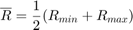
Fig. 8 shows the ratio of the optimal time allocated to the far user over that to the near user , i.e.,  in (P1) versus (P2), with different values of the common pathloss exponent in both DL and UL, where the same two-user channel setup as for Fig. 5 is considered. It is assumed that for the near user is fixed as and
  for the far user is set the same as for Fig. 6. For P1, we can find the optimal based on Proposition 3.1
R_p1 = zeros(1, N);
for i = 1 : N
    tau_opt = Optimal_tau_func_pro3(K, [gamma1_wpcn, gamma2_wpcn(i)]);
    R_p1(i) = tau_opt(3)/tau_opt(2); % the ratio of tau2 / tau1
end

% For P2, we can use the iterative optimization algorithm to optimize tau
R_p2 = zeros(1, N);
for i = 1 : N
    gamma = [gamma1_wpcn,gamma2_wpcn(i)];
    [tau_opt, R_tau, lambda] = optimal_tau_cal(K, gamma);
    R_p2(i) = tau_opt(3)/tau_opt(2);
end

figure
semilogy(alpha,R_p1, 'r-o ', alpha,R_p2, 'b-d ', 'linewidth',2)
xlabel('Pathloss Exponent(\alpha)','fontsize',12);
ylabel('\tau^*_2 / \tau^*_1','fontsize',12);
legend('(P1)','(P2)');
grid on
title('Fig. 8 in the Paper (Iterative Algorithm)')
However, the figure is not exactly the same with Fig. 8 in the paper. A possible reason is that the convergence performance of the algorithm here may be different from that implemented in the original paper. We tried to find the optimal value of by using brute force algorithm, and the obtained figure is almost identical with Fig. 8 in the paper.
% For P2, using the brute force algorithm to find the optimal tau
R_p2_bf = zeros(1, N);
for i = 1 : N
    gamma = [gamma1_wpcn,gamma2_wpcn(i)];
    [R_tau, tau_opt] =  Brute_force(K, gamma, 0.01, 2);
    R_p2_bf(i) = tau_opt(3)/tau_opt(2);
end

figure
semilogy(alpha,R_p1, 'r-o ', alpha,R_p2_bf, 'b-d ', 'linewidth',2)
xlabel('Pathloss Exponent(\alpha)','fontsize',12);
ylabel('\tau^*_2 / \tau^*_1','fontsize',12);
legend('(P1)','(P2)');
grid on
title('Fig. 8 in the Paper (Brute Force Algorithm)')
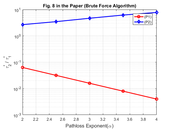
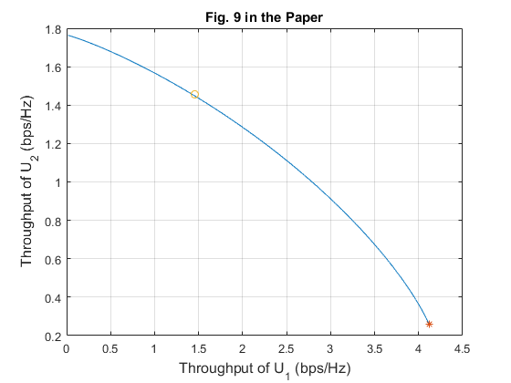
Fig. 9 shows the achievable throughput region of a two-user WPCN by solving the weighted sum-throughput maximization problem in (15) with different throughput weights for the near and far users, under the same channel setup as for Fig. 5. In the figure, "*" corresponds to the maximum sum-throughput and "o" corresponds to the maximum common-throughput.
[tau_2,tau_1] = meshgrid(0.001:0.001:1);
N_9 = length(tau_1);
R_o1 = zeros(1, N_9);
R_o2 = zeros(1, N_9);
% plot the achievable throughput region of the two-user WPCN
for i = 1:N_9
    R_temp = R_sum_5(:, 1:i);
    [m,n] = find(R_temp == max(max(R_temp)));
    R_o1(i) = R1_5(m,n);
    R_o2(i) = R2_5(m,n);
end

figure
plot(R_o1, R_o2)
hold on
% plot the solution of P1 (obtained in Fig 5)
plot(R1_opt_5,R2_opt_5,'*');
hold on
% plot the solution of P2 (obtained in Fig 7)
plot(R1_opt_7,R2_opt_7,'o');
hold on
grid on;
xlabel('Throughput of U_1 (bps/Hz)','fontsize',12);
ylabel('Throughput of U_2 (bps/Hz)','fontsize',12);
title('Fig. 9 in the Paper');
Data Sources
In the simulation part, it is assumed that the channel reciprocity holds for the DL and UL and thus  , with the same pathloss exponent . Accordingly, both the DL and UL channel power gains are modeled as
  , where
  represents the additional channel short-term fading which is assumed to be Rayleigh distributed, and
  is an exponentially distributed random variable with unit mean. The values of parameters are shown in the following table,
| Parameter | Value |
| Bandwidth | 1 MHz |
| Additional channel short-term fading | Rayleigh distribution |
| Average signal power attenuation | 30dB |
| AWGN at the H-AP receiver | -160dBm/Hz |
| Signal-to-noise ratio (SNR) gap | 9.8dB |
| Energy harvesting efficiency for WET | 0.5 |
Visualization of Results
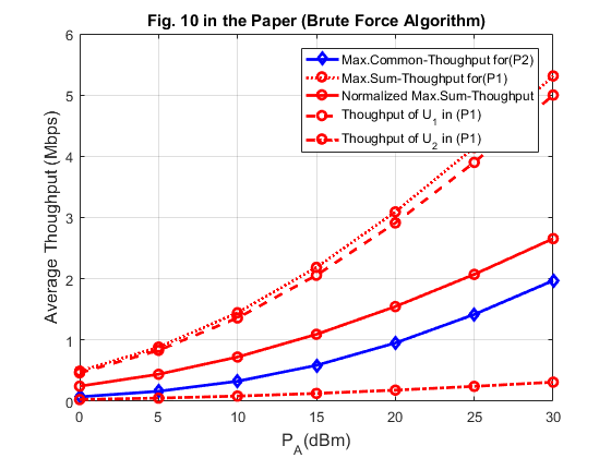
Fig. 10 shows the maximum sum-throughput versus the maximum common-throughput in the same WPCN with ,  , and
, and  for different values of transmit power at H-AP, PA, in dBm.
K = 2; % number of users
xi = 0.5; % energy harvesting efficiency
Gamma  = 9.8; % SNR gap, dB
D1 = 5; % distance from user i to the AP
D2 = 10;
alpha = 2; % channel pathloss exponent
sigma_1 = -160; % noise power spectral density, dBm/HZ;
sigma = -160 + 10*log10(10^6); % noise power, dBm;
Considering that it takes a long time for the iterative algorithm to converge, we do not average over 1000 randomly generated fading channel realizations as stated in the paper. Instead, we take the mean value of the fading, i.e.,  , in this part.
h_1 = 10^(-3)*D1^(-alpha);
g_1 = 10^(-3)*D1^(-alpha);
h_2 = 10^(-3)*D2^(-alpha);
g_2 = 10^(-3)*D2^(-alpha);
PA = 0:5:30;
N_PA = length(PA);
gamma1 = xi*h_1*g_1*10.^(PA./10)/(10^((Gamma+sigma)/10));
gamma2 = xi*h_2*g_2*10.^(PA./10)/(10^((Gamma+sigma)/10));

R_o1_p1 = zeros(1, N_PA); R_o2_p1 = zeros(1, N_PA); R_sum_o2_p1 = zeros(1, N_PA);
R_sum_Norm_p1 = zeros(1, N_PA);
R_o1_p2 = zeros(1, N_PA); R_o2_p2 = zeros(1, N_PA); R_min = zeros(1, N_PA);
for i = 1 : N_PA
    % for P1, we can find the optimal tau based on Proposition 3.1
    gamma_p = [gamma1(i),gamma2(i)];
    [tau_p1] = Optimal_tau_func_pro3(K, gamma_p);
    R_o1_p1(i) =  tau_p1(2)*log2(1+gamma1(i)*tau_p1(1)/tau_p1(2));
    R_o2_p1(i) =  tau_p1(3)*log2(1+gamma2(i)*tau_p1(1)/tau_p1(3));
    R_sum_o2_p1(i) = R_o1_p1(i) + R_o2_p1(i);
    R_sum_Norm_p1(i) = R_sum_o2_p1(i)/K;

    % for P2, using the iterative algorithm to obtain the optimal solution
    [tau_opt, R_tau, lambda] = optimal_tau_cal(K, gamma_p);
    R_o1_p2(i) =  R_tau(1);
    R_o2_p2(i) =  R_tau(2);
    R_min(i) = min(R_tau);
end
figure
plot(PA,R_min,'-db',PA,R_sum_o2_p1,':or',PA,R_sum_Norm_p1,'-or',PA,R_o1_p1,'--or',PA,R_o2_p1,'-.or','linewidth',2);
xlabel('P_A(dBm)','fontsize',12);
ylabel('Average Thoughput (Mbps)','fontsize',12);
legend('Max.Common-Thoughput for(P2)','Max.Sum-Thoughput for(P1)','Normalized Max.Sum-Thoughput',...
    'Thoughput of U_1 in (P1)','Thoughput of U_2 in (P1)');
grid on;
title('Fig. 10 in the Paper (Iterative Algorithm)');
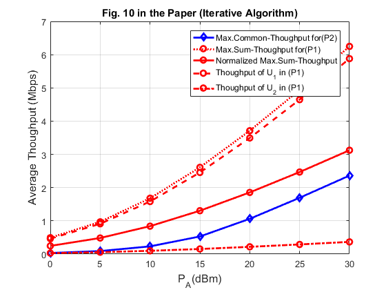
The achievable throughput is generally larger than that shown in the paper. A possible reason is that we ignored the impact of fast fading. To consider the impact of the fading, we can use the brute borce algorithm and average over 1000 randomly generated fading channel realizations, we can obtain almost identical figure as Fig 10 in the paper.
num_rand = 1000;
R_o1_p1 = zeros(num_rand, N); R_o2_p1 = zeros(num_rand, N); R_sum_o2_p1 = zeros(num_rand, N);
R_sum_Norm_p1 = zeros(num_rand, N);
R_min = zeros(num_rand, N);

for iter_rand = 1: num_rand
    rho = exprnd(1);

    h_1 = 10^(-3)*rho*D1^(-alpha);
    g_1 = 10^(-3)*rho*D1^(-alpha);
    h_2 = 10^(-3)*rho*D2^(-alpha);
    g_2 = 10^(-3)*rho*D2^(-alpha);
    gamma1 = xi*h_1*g_1*10.^(PA./10)/(10^((Gamma+sigma)/10));
    gamma2 = xi*h_2*g_2*10.^(PA./10)/(10^((Gamma+sigma)/10));

    for i = 1 : N_PA
        % for P1, we can find the optimal tau based on Proposition 3.1
        gamma_p1 = [gamma1(i),gamma2(i)];
        [tau_p1] = Optimal_tau_func_pro3(K, gamma_p1);
        R_o1_p1(iter_rand, i) =  tau_p1(2)*log2(1+gamma1(i)*tau_p1(1)/tau_p1(2));
        R_o2_p1(iter_rand, i) =  tau_p1(3)*log2(1+gamma2(i)*tau_p1(1)/tau_p1(3));
        R_sum_o2_p1(iter_rand, i) = R_o1_p1(iter_rand, i) + R_o2_p1(iter_rand, i);
        R_sum_Norm_p1(iter_rand, i) = R_sum_o2_p1(iter_rand, i)/2;

        % for P2, using the brute force algorithm to obtain the optimal solution
        [R_max, tau_opt] = Brute_force(K, gamma_p1, 0.02, 2);
        R_min(iter_rand, i) = min(R_max);
    end
end

figure
plot(PA,mean(R_min),'-db',PA,mean(R_sum_o2_p1),':or',PA,mean(R_sum_Norm_p1),'-or',PA,mean(R_o1_p1),'--or',PA,mean(R_o2_p1),'-.or','linewidth',2);
xlabel('P_A(dBm)','fontsize',12);
ylabel('Average Thoughput (Mbps)','fontsize',12);
legend('Max.Common-Thoughput for(P2)','Max.Sum-Thoughput for(P1)','Normalized Max.Sum-Thoughput',...
    'Thoughput of U_1 in (P1)','Thoughput of U_2 in (P1)');
grid on
title('Fig. 10 in the Paper (Brute Force Algorithm)');
By fixing  , Fig. 11 shows the throughput comparison for different values of the common pathloss exponent in both the DL and UL in the same WPCN as for Fig.10.
PA = 20;
alpha = 2:0.5:4;
N_alpha = length(alpha);

% Channel power gains
h_1 = 10^(-3)*D1.^(-alpha);
g_1 = 10^(-3)*D1.^(-alpha);
h_2 = 10^(-3)*D2.^(-alpha);
g_2 = 10^(-3)*D2.^(-alpha);
gamma1 = xi.*h_1.*g_1*10^(PA/10)/(10^((Gamma+sigma)/10));
gamma2 = xi.*h_2.*g_2*10^(PA/10)/(10^((Gamma+sigma)/10));

R_o1_p1 = zeros(1, N_alpha); R_o2_p1 = zeros(1, N_alpha); R_sum_o2_p1 = zeros(1, N_alpha);
R_sum_Norm_p1 = zeros(1, N_alpha);
R_o1_p2 = zeros(1, N_alpha); R_o2_p2 = zeros(1, N_alpha); R_min = zeros(1, N_alpha);
for i = 1 : N_alpha
    gamma_p1 = [gamma1(i),gamma2(i)];
    % for P1, we can find the optimal tau based on Proposition 3.1
    [tau_p1] = Optimal_tau_func_pro3(K,gamma_p1);
    R_o1_p1(i) =  tau_p1(2)*log2(1+gamma1(i)*tau_p1(1)/tau_p1(2));
    R_o2_p1(i) =  tau_p1(3)*log2(1+gamma2(i)*tau_p1(1)/tau_p1(3));
    R_sum_o2_p1(i) = R_o1_p1(i) + R_o2_p1(i);
    R_sum_Norm_p1(i) = R_sum_o2_p1(i)/2;

    % for P2,  using the iterative algorithm to obtain the optimal solution
    [tau_opt, R_tau, lambda] = optimal_tau_cal(K, gamma_p1);
    R_o1_p2(i) =  R_tau(1);
    R_o2_p2(i) =  R_tau(2);
    R_min(i) = min(R_tau);
end

figure
plot(alpha,R_min,'-db',alpha,R_sum_o2_p1,':or',alpha,R_sum_Norm_p1,'-or',alpha,R_o1_p1,'--or',alpha,R_o2_p1,'-.or','linewidth',2);
xlabel('Pathloss Exponent(\alpha)','fontsize',12);
ylabel('Average Thoughput(Mbps)','fontsize',12);
legend('Max.Common-Thoughput for(P2)','Max.Sum-Thoughput for(P1)','Normalized Max.Sum-Thoughput',...
    'Thoughput of U_1 in (P1)','Thoughput of U_2 in (P1)');
grid on
title('Fig. 11 in the Paper (Iterative Algorithm)');
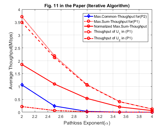
Similarly, the achievable performance is generally larger than the results given in the paper. To simulate the impact of channel fading, we can use the brute force algorithm and average over 1000 randomly generated fading channel realizations
num_rand = 1000;
R_o1_p1 = zeros(num_rand, N_alpha); R_o2_p1 = zeros(num_rand, N_alpha); R_sum_o2_p1 = zeros(num_rand, N_alpha);
R_sum_Norm_p1 = zeros(num_rand, N_alpha);
R_min = zeros(num_rand, N_alpha);

for iter_rand = 1: num_rand
    rho = exprnd(1);

    h_1 = 10^(-3)*rho*D1.^(-alpha);
    g_1 = 10^(-3)*rho*D1.^(-alpha);
    h_2 = 10^(-3)*rho*D2.^(-alpha);
    g_2 = 10^(-3)*rho*D2.^(-alpha);
    gamma1 = xi.*h_1.*g_1*10^(PA/10)/(10^((Gamma+sigma)/10));
    gamma2 = xi.*h_2.*g_2*10^(PA/10)/(10^((Gamma+sigma)/10));

    for i = 1 : N_alpha
        gamma_p1 = [gamma1(i),gamma2(i)];
        % for P1, we can find the optimal tau based on Proposition 3.1
        [tau_p1] = Optimal_tau_func_pro3(K,gamma_p1);
        R_o1_p1(iter_rand, i) =  tau_p1(2)*log2(1+gamma1(i)*tau_p1(1)/tau_p1(2));
        R_o2_p1(iter_rand, i) =  tau_p1(3)*log2(1+gamma2(i)*tau_p1(1)/tau_p1(3));
        R_sum_o2_p1(iter_rand, i) = R_o1_p1(iter_rand, i) + R_o2_p1(iter_rand, i);
        R_sum_Norm_p1(iter_rand, i) = R_sum_o2_p1(iter_rand, i)/2;

        % for P2, using the brute force algorithm to obtain the optimal solution
        [R_max, tau_opt] = Brute_force(K, gamma_p1, 0.02, 2);
        R_min(iter_rand, i) = min(R_max);
    end
end

figure
plot(alpha,mean(R_min),'-db',alpha,mean(R_sum_o2_p1),':or',alpha,mean(R_sum_Norm_p1),...
    '-or',alpha,mean(R_o1_p1),'--or',alpha,mean(R_o2_p1),'-.or','linewidth',2);
xlabel('Pathloss Exponent(\alpha)','fontsize',12);
ylabel('Average Thoughput(Mbps)','fontsize',12);
legend('Max.Common-Thoughput for(P2)','Max.Sum-Thoughput for(P1)','Normalized Max.Sum-Thoughput',...
    'Thoughput of U_1 in (P1)','Thoughput of U_2 in (P1)');
grid on
title('Fig. 11 in the Paper (Brute Force Algorithm)');
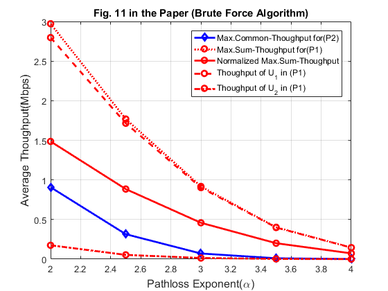
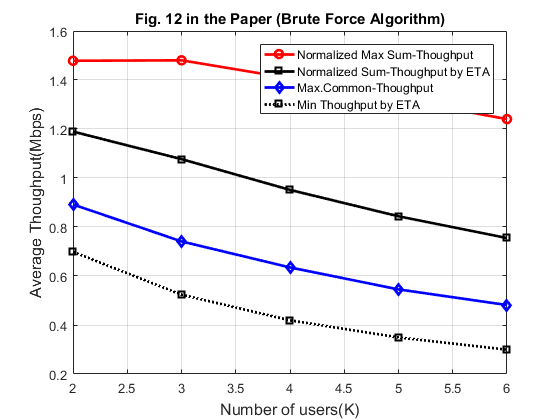
Fig. 12 shows the throughput over number of users, . It is assumed that users in the network are equally separated from the H-AP according to  ,
,  , where
  . The transmit power at the H-AP and the pathloss exponent are set to be fixed as and
  , respectively. In addition, the authors also compare with the throughput achievable by equal time allocation (ETA), i.e.,
 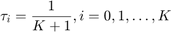 , as a lowcomplexity time allocation scheme.
alpha = 2;
DK = 10;
PA = 20;
K_1 = 2:1:6;
N_K = length(K_1);

% calculate gamma with different numbers of users
gamma = cell(1, N_K);
for j = 1 : N_K
    gamma{j} = zeros(1, j);
    for z = 1 : j+1
        D = DK/(j+1)*z;
        h = 10^(-3)*D^(-alpha);
        g = 10^(-3)*D^(-alpha);
        gamma{j}(z) = xi*h*g*10^(PA/10)/(10^(Gamma/10)*10^(sigma/10));
    end
end

% Normalized Max sum-thoughput P1
R_Norm_max = zeros(1, N_K);
for j = 2:1:6
    % For max sum-throughput (P1), optimize based on Proposition 3.1
    [tau_p1] = Optimal_tau_func_pro3(j,gamma{j-1});
    R_o_p1 = zeros(1, j);
    for i=1:j
        R_o_p1(i) = tau_p1(i+1)*log2(1+gamma{j-1}(i)*tau_p1(1)/tau_p1(i+1));
    end
    R_Norm_max(j-1) = sum(R_o_p1)/j;
end

% Max. Common-throughput P2
R_max_common = zeros(1, N_K);
for j = 2:1:6
    % use the iterative algorithm to maximize the common throughput
    [tau_p2, R_tau, lambda] = optimal_tau_cal(j, gamma{j-1});
    R_o_p2 = zeros(1, j);
    for i=1:j
        R_o_p2(i) = tau_p2(i+1)*log2(1+gamma{j-1}(i)*tau_p2(1)/tau_p2(i+1));
    end
    R_max_common(j-1) = min(R_o_p2);
end

% Equal time allocation
R_min_eta = zeros(1, N_K);
R_norm_eta = zeros(1, N_K);
for i = 1 : N_K
    R = zeros(1, K_1(i));
    for z = 1 : K_1(i)
        tau = 1 / (K_1(i)+1);
        R(z) = tau * log2(1 + gamma{i}(z));
    end
    R_min_eta(i) = min(R);
    R_norm_eta(i) = sum(R)/K_1(i);
end

figure;
plot(K_1,R_Norm_max,'-or', K_1,R_norm_eta,'-sk', K_1,R_max_common,'-db', K_1,R_min_eta,':sk', 'linewidth',2);
xlabel('Number of users(K)','fontsize',12);
ylabel('Average Thoughput(Mbps)','fontsize',12);
legend('Normalized Max Sum-Thoughput','Normalized Sum-Thoughput by ETA','Max.Common-Thoughput','Min Thoughput by ETA');
grid on
title('Fig. 12 in the Paper (Iterative Algorithm)');

Similarly, we can have the resultes obtained by brute force algorithm.
num_rand = 1000;
R_Norm_max = zeros(num_rand, N_K); R_max_common = zeros(num_rand, N_K);
R_min_eta = zeros(num_rand, N_K); R_norm_eta = zeros(num_rand, N_K);

for iter_rand = 1: num_rand
    rho = exprnd(1);

    % calculate gamma with different numbers of users
    gamma = cell(1, N_K);
    for j = 1 : N_K
        gamma{j} = zeros(1, j);
        for z = 1 : j+1
            D = DK/(j+1)*z;
            h = 10^(-3)*rho*D^(-alpha);
            g = 10^(-3)*rho*D^(-alpha);
            gamma{j}(z) = xi*h*g*10^(PA/10)/(10^(Gamma/10)*10^(sigma/10));
        end
    end

    % Normalized Max sum-thoughput P1
    for j = 2:1:6
        [tau_p1] = Optimal_tau_func_pro3(j,gamma{j-1});
        R_o_p1 = zeros(1, j);
        for i=1:j
            R_o_p1(i) = tau_p1(i+1)*log2(1+gamma{j-1}(i)*tau_p1(1)/tau_p1(i+1));
        end
        R_Norm_max(iter_rand, j-1) = sum(R_o_p1)/j;
    end

    % Max. Common-throughput P2, using brute force algorithm
    for j = 1 : N_K
        [R_max, tau_opt] = Brute_force(K_1(j), gamma{j}, 0.05, 2);
        R_max_common(iter_rand, j) = R_max;
    end

    % Equal time allocation
    for i = 1 : N_K
        R = zeros(1, K_1(i));
        for z = 1 : K_1(i)
            tau = 1 / (K_1(i)+1);
            R(z) = tau * log2(1 + gamma{i}(z));
        end
        R_min_eta(iter_rand, i) = min(R);
        R_norm_eta(iter_rand, i) = sum(R)/K_1(i);
    end

end

figure
plot(K_1,mean(R_Norm_max),'-or', K_1,mean(R_norm_eta),'-sk', K_1,mean(R_max_common),'-db', K_1,mean(R_min_eta),':sk', 'linewidth',2);
xlabel('Number of users(K)','fontsize',12);
ylabel('Average Thoughput(Mbps)','fontsize',12);
legend('Normalized Max Sum-Thoughput','Normalized Sum-Thoughput by ETA','Max.Common-Thoughput','Min Thoughput by ETA');
grid on
title('Fig. 12 in the Paper (Brute Force Algorithm)');
Analysis and Conclusions
1. The two proposed maximization problems, i.e.,sum-throughput maximization problem (P1) and common-throughput maximization problem (P2), are reproduced. We were able to reprodece all of the results figures presented in the original paper [1].
2. For problem (P1), the authors have given out a closed form of the solution and shown the corresponding proofs. In this report, we also use the brute force method to solve the original problem (P1) to further show the correctness of the provided closed form expression. For problem (P2), the authors have mentioned to use sub-gradient based algorithms to update in their proposed algorithm, thus, we choose the gradient descent method to realize the provided algorithm in this report. Our simulation results have shown the correctness of the original simulation results.
3. However, for problem (P2), we noticed that the running time of the proposed iterative algorithm is  or more times longer than the brute force method. One-time simulation of the proposed iterative algorithm lasts for hours, while only 10 minutes are required for the brute force method. Thus, for Fig.10 - 12, instead of showing the results by averaging over 1000 randomly generated fading channel realizations as the authors mentioned in the paper, we have shown the results of one-time simulation of the proposed iterative algorithm and also shown the results of using brute force algorithm and averaging over 1000 times. Moreover, we also noticed that, the iterative algorithm implemented in this project converges to a better result than that given in the paper, although it may take a longer time.
References
[1] Hyungsik Ju and Rui Zhang, `Throughput Maximization in Wireless Powered Communication Networks', IEEE Trans. Wireless Commun., vol.13, no. 1, pp. 418-428, 2014.
Print all the functions used in the project
type('Optimal_tau_func_pro3')
function [tau] = Optimal_tau_func_pro3(k, gamma)
% This function calculates optimal tau by proposition 3.1
A = sum(gamma);
syms z
z_1 = solve( z*log(z)- z + 1 == A,z);
z = eval(z_1);
tau = zeros(1, k + 1);
tau(1) = (z - 1)/(A + z -1);
for i = 1 : k
    tau(i + 1) = gamma(i)/(A + z -1);
end
type('optimal_tau_cal')
function [tau_opt, R_tau, lambda] = optimal_tau_cal(k, gamma)
% This function optimizes the value of tau to obtained the maximum common
% throughput, according to the algorithm in Table I in the paper

R_min = 0; R_max = 1e2;
lambda = 1 ./ log10(1+gamma); % initialize the value of lambda

% calculate the optimal values of z and tau based on Proposition 4.1
[R_tau, tau_opt] = tau_opt_cal(k, lambda, gamma);

delta = 1e-3;
tau = 0.01;
while R_max - R_min > delta
    flag_R_aver = 0;
    while flag_R_aver == 0
        R_aver = mean([R_min, R_max]);
        g_lambda = - sum(lambda .* R_tau) + sum(lambda) * R_aver; % compute g(lambda)

        if g_lambda > 0 % R_aver is infeasible, decrease R_aver
            R_max = R_aver;
            if R_max - R_min <= delta
                flag_R_aver =1;
            end
        elseif g_lambda <=0
            % update the value of lambda by using the gradient descent algorithm
            [tau, lambda, R_tau, tau_opt] = gradient_descent(tau, lambda, k, R_tau, R_aver, gamma);
            g_lambda = - sum(lambda .* R_tau) + sum(lambda) * R_aver; % compute g(lambda)
            if g_lambda <= 0
                R_min = R_aver;
            end
            flag_R_aver = 1;
        end

    end
end
type('tau_opt_cal')
function [R_tau, tau_opt] = tau_opt_cal(k, lambda, gamma)
% This function calculates the optimal values of z and tau based on Proposition 4.1

u_min = 0; u_max = 1e1;
flag = 0;

% first find the optimal value of u and z based on known lambda and gamma
while flag == 0
    u = mean([u_min, u_max]);
    z_opt = zeros(1, k);

    for i = 1 : k
        syms x
        % find the value of z satisfying equation (18) in the paper
        z_opt(i) = solve(log(1+x) - x/1+x == u/lambda(i) * log(2), x);
    end

    % calculate the value of the left-hand side of (19)
    s_z = sum(lambda .* gamma ./ (1 + z_opt));
    if abs(s_z - u * log(2)) <= 1e-3 % if equation (19) holds
        flag = 1;
    elseif s_z < u * log(2)
        u_max = u;
    elseif s_z > u * log(2)
        u_min = u;
    end
end

% based on the obtained u and z, calculate the optimal tau based on Proposition 4.1
tau_opt = zeros(1, k+1);
tau_opt(1) = 1 / ( 1 + sum(gamma./z_opt) );
R_tau = zeros(1, k);
for i = 1 : k
    tau_opt(i+1) = gamma(i) / z_opt(i) / (1 + sum(gamma./z_opt) );
    if tau_opt(i+1) == 0
        R_tau(i)  = 0;
    else
        R_tau(i) = tau_opt(i+1) * log2(1 + gamma(i) * tau_opt(1) / tau_opt(i+1));
    end
end
type('gradient_descent')
function [tau, x, R_tau, tau_opt] = gradient_descent(tau, lambda, k, R_tau, R_aver, gamma)
% This function updates the value of lambda by using gradient descent

x = 10 * ones(1, k);
x_new = lambda; % x_new = initial value of lambda
fun_g_new = sum(x_new .* R_tau) - sum(x_new) * R_aver;
fun_g = inf;
epsilon = 1e-2;
step = 0;

while abs(fun_g_new - fun_g) > epsilon * abs(fun_g_new)
    x = x_new;
    step = step + 1;
    if rem(step, 10) ==0
        tau = tau /2;
    end
    fun_g = fun_g_new;

    g = R_tau - R_aver; % the gradient of g(lambda) over lambda
    x_new = x - tau * g; % update the value of x_new
    x_new = max(x_new, 1e-3);
    % based on newly obtained value of lambda (here is x_new), update the
    % optimal valuse of tau, R(tau), and R_aver, which are related to the
    % gradient of g(lamda) in x_new
    [R_tau, tau_opt] = tau_opt_cal(k, x_new, gamma);
    fun_g_new = sum(x_new .* R_tau) - sum(x_new) * R_aver;
end
type('Brute_force')
function [R_max, tau_opt] = Brute_force(k, gamma, step, flag)
% this function finds the optimal value of tau by using brute force
% flag = 1 indicates that we want to solve the max sum-throughput problem;
% flag = 2 indicates that we want to maximize the common throughput

tau = zeros(1, k);
num = 1 / step + 1;
R_max = 0;
for i = 1 : num^k - 1
    % generate the values of tau for all the k users
    tau(1) = floor(i/num^(k - 1));
    step_sum = 0;
    for j = 2 : k
        step_sum = step_sum + tau(j-1)*num^(k - j + 1);
        tau(j) = floor((i - step_sum)/num^(k - j));
    end
    tau =tau*step;
    % for tau0 > 0 and tau_i > 0 for all the users, calculate the
    % corresponding throughput
    if sum(tau) < 1
        tau0 = 1 - sum(tau);
        R = zeros(1, k);
        for m = 1 : k
            if tau(m) ~= 0
                R(m) = tau(m)*log2(1+gamma(m)*tau0/tau(m));
            end
        end
        % find the optimal tau which leads to the optimal sum or common throughput
        if flag == 1 && sum(R) > R_max
            R_max = sum(R);
            tau_opt = [tau0, tau];
        elseif flag == 2 && min(R) > R_max
            R_max = min(R);
            tau_opt = [tau0, tau];
        end
    end
end