Fast large-scale optimization by unifying stochastic gradient and quasi-Newton methods
Contents
- Group Members
- 1. Project Discription
- 2. Formal Definition of Objective Function in Autoencoder
- 3. Overall Design Sum of Functions Optimizer
- 3.1 Approximating the objective function
- 3.2 Get an Estimate of Subfunction
- 3.3 Subspace Update
- 3.4 Online Hessian Approximation
- 3.5 Detecting bad updates
- 3.6 Growing the number of active subfunctions
- 3.7 Perform One Step Optimization
- 4. Set Up Hyperparameters
- 5. Data Import
- 6. Optimize Autoencoder Using SFO on MNIST Dataset
- 6.1 Reconstruction of Autoencoder Trained by SFO
- 7. Optimize Autoencoder Using Other Optimizers On MNIST Dataset
- 7.1 Reconstruction of Autoencoder Trained by lbfgs
- 8. Analysis and conclusions
- References
Group Members
ECE602: Introduction to Optimization (Winter, 2018)
Group Members: Lingheng Meng, 20702336; Ala Eldin Omer, 20738888 Daiwei Lin, 20490018;
1. Project Discription
In this project, we will reimplememt Sum of Functions (SFO) optimizer proposed in [1], then test the optimizer in optimizing an Autoencoder on synthetic data, and compared its performance against lbfgs.
Autoencoder is a basic neural netorwork model intending to automatically abstract features from original data. The classic structure of Autoencoder is a two layer NN that has a input layer, a hidden layer and a output layer. The objective of Autoendocer is to reconstruct input on the output layer i.e. optimizing objective function to let 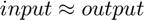 .
.
With stacking, greedy-layerwise training and fine-tuning strategies, Autoencoder could act as a block to construct deep neural network.
In this project, we reproduce result on Autoencoder as illustrated in paper [1].
2. Formal Definition of Objective Function in Autoencoder
In this section, we will illustrate the formal experssion of objective function and derive the back-propagated gradient with respect to each parameter in an Autoencoder.
Forward Propagation (for each datapoint) :

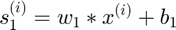
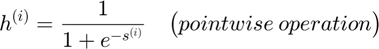
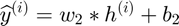
Objective Function (for all datapoints in a batch):
Back-Propagation of Gradient (for each datapoint):

The forward and backward propagation we derived here will be incorporated in a single function called f_df_autoencoder. And this function wil be called in SFO optimizer.
The optimization problem can be expressed as:
function [f, dfdtheta] = f_df_autoencoder(theta, v)
    % [f, dfdtheta] = f_df_autoencoder(theta, v)
    %     Calculate L2 reconstruction error and gradient for an autoencoder
    %     with sigmoid nonlinearity.
    %     Parameters:
    %         theta - A cell array containing
    %              {[weight matrix], [hidden bias], [visible bias]}.
    %         v - A [# visible, # datapoints] matrix containing training data.
    %              v will be different for each subfunction.
    %     Returns:
    %         f - The L2 reconstruction error for data v and parameters theta.
    %         df - A cell array containing the gradient of f with each of the
    %              parameters in theta.
    cell_para = 0;
    if iscell(theta)
        cell_para = 1;
        W = theta{1};
        b_h = theta{2};
        b_v = theta{3};
    else
    	M = 784;
        J=50;
        W = reshape(theta(1:J*M),J,M);
        b_h = reshape(theta(J*M+1:(J*M+J)),J,1);
        b_v = reshape(theta(((J*M+J)+1):end),M,1);
    end


    h = 1./(1 + exp(-bsxfun(@plus, W * v, b_h)));
    v_hat = bsxfun(@plus, W' * h, b_v);
    f = sum(sum((v_hat - v).^2)) / size(v, 2);
    dv_hat = 2*(v_hat - v) / size(v, 2);
    db_v = sum(dv_hat, 2);
    dW = h * dv_hat';
    dh = W * dv_hat;
    db_h = sum(dh.*h.*(1-h), 2);
    dW = dW + dh.*h.*(1-h) * v';
    % give the gradients the same order as the parameters
    if cell_para == 1
        dfdtheta = {dW, db_h, db_v};
    else
        dfdtheta = [dW(:); db_h(:); db_v];
    end
end
3. Overall Design Sum of Functions Optimizer
In this section, we are going to illustrate the underlying mehodology to implememt SFO using a MATLAB code.
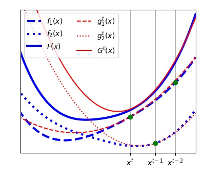
3.1 Approximating the objective function
A series of functions  (sum of N subfunctions
  each of whcih is a quadratic approximation to its corresponding
  ) is defined to approximate the objective function
  in each learning iteration as shown in the Figure below. The functions will be stored and one of them is updated every learning step t:
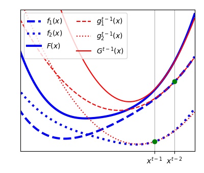
i. A vector  is chosen as shown in the Figure below by minimizing the approximated objective function
  at the previous iteration by a Newton step.
 $ Equation(4)

ii. Only one subfunction  of index
  is chosen (to be updated) according to Equation (13), that is last evaluated farthest from current location (least accurate)
![$$ j= argmax_{i} [x^{t}-x^{\tau_{i}}]^{T} Q^{t} [x^{t}-x^{\tau_{i}}] $$](main_eq08851176493750539182.png) Equation (13)
Equation (13)
where  is the time at which subfunction
  was last evaluated and Q is set either to approximated Hessian for this subfunction (more accurate measure of distance) or full Hessian to avoid bad Hessian estimate for a single subfunction (evaluation impossible).
function indx = get_target_index(obj)
% Choose which subfunction to update in certain learning iteration
    gd = find((obj.eval_count < 2) & obj.active);  % If an active subfunction has less than two observations, then
% evaluate it again. Two evaluations per subfunction are needed to estimate its Hessian;
    if ~isempty(gd)
        indx = gd(randperm(length(gd), 1));
        return
    end
    % choose the subfunction evaluated farthest using either total weighted Hessian, or by the subfunction Hessian
    if randn() < 0
        max_dist = -1;
        indx = -1;
        for i = 1:obj.N
            dtheta = obj.theta_proj - obj.last_theta(:,i);
            bdtheta = obj.b(:,:,i).' * dtheta;
            dist = sum(bdtheta.^2) + sum(dtheta.^2)*obj.min_eig_sub(i);
            if (dist > max_dist) && obj.active(i)
                max_dist = dist;
                indx = i;
            end
        end
    else
        dtheta = bsxfun(@plus, obj.theta_proj, -obj.last_theta); % difference between current theta & all subfunctions recent evaluation;
        full_H_combined = obj.get_full_H_with_diagonal(); % full Hessian;
        distance = sum(dtheta.*(full_H_combined * dtheta), 1); % squared distance;
        [~, dist_ord] = sort(-distance); % sort the distances from largest to smallest;
        dist_ord = dist_ord(obj.active(dist_ord)); % keep indices of active subfunctions;
        indx = dist_ord(1); % choose the active subfunction that is farthest from current location;;
    end
end
3.2 Get an Estimate of Subfunction
The chosen subfunction of index ( ) is updated (as shown in the Figure below for
  ) using a second order power series (Equation (6)) around the vector chosen in the step (i).
 Equation (6)
where the quadratic term  is the Hessian of this subfunction and is approximated using BFGS algorithm based on its history of grdaient evaluation (details in step 3.4)
function f_pred = get_predicted_subf(obj, indx, theta_proj)
% Get the predicted value of subfunction indx at theta_proj that lies insisde the subspace;
    dtheta = theta_proj - obj.last_theta(:,indx);
    bdtheta = obj.b(:,:,indx).' * dtheta;
    Hdtheta = real(obj.b(:,:,indx) * bdtheta);
    Hdtheta = Hdtheta + dtheta.*obj.min_eig_sub(indx); % the diagonal contribution
    f_pred = obj.hist_f(indx,1) + obj.last_df(:,indx).' * dtheta + 0.5.*(dtheta.') * (Hdtheta);
end
3.3 Subspace Update
The subspace is expanded at each optimization step t to include the most recent gradient direction as an additional column by finding the gradient vector component that lies outside the exsiting subspace and appending it to the current subspace. Following equations were used:
 Equation (7)
![$$ P^{t}=\left [P^{t-1} \frac{q_{orth}}{\left \|q_{orth}\right\|}\right] $$](main_eq11207303121271640830.png) Equation (8)
Equation (8)
i. The function update_subspace(obj, x_in) is written to update the subspace at each optimization step t to include the most recent gradient direction as an additional column. This is done by finding the gradient vector component that lies outside the exsiting subspace and appending it to the current subspace.
function update_subspace(obj, x_in)
% Update the low dimensional subspace by adding a new gradient direction x_in to be incorporated into the subspace.;
    if obj.K_current >= obj.M
        return; % no need to update the subspace if it spans the full space;
    end
    if sum(~isfinite(x_in)) > 0
        return; % bad vector!
    end
    x_in_length = sqrt(sum(x_in.^2));
    if x_in_length < obj.eps
        return; % nothing to do with a short new vector
    end
    xnew = x_in/x_in_length; % make x unit length;
    % Find the component of x pointing out of the existing subspace.;
    % This is done multiple times for numerical stability.;
    % $$ q_{orth}=f_{j}^{'}(x^{t})-P^{t-1}(P^{t-1})^{T} f_{j}^{'}(x^{t}) $$  Equation (7)
    for i = 1:3
        xnew = xnew - obj.P * (obj.P.'*xnew);
        ss = sqrt(sum(xnew.^2));
        if ss < obj.eps % barely points out of the existing subspace
            return; % no need to add a new direction to the subspace;
        end
        xnew = xnew / ss; % make it unit length;
        if ss > 0.1 % largely orthogonal >> good numerical stability
            break;
        end
    end
    % update the subspace with a new column containing the new direction;
    % $$ P^{t}=\left [P^{t-1} \frac{q_{orth}}{\left \|q_{orth}\right\|}\right] $$ Equation (8)
    obj.P(:,obj.K_current+1) = xnew;
    obj.K_current = obj.K_current + 1;

% Restricting the size of the subspace: In case the subspace dimensionality K^{t} exceeds K_{max}, it is collapsed to a new subspace
% that includes only the most recent gradient and position measurements from each subfunction through QR decomposition
    if obj.K_current >= obj.K_max
    % collapse the subspace when it exceeded its maximum allowed size
    % xl is passed explicity to make sure it's used if not in
    % history yet.
        xl = (obj.P.') * (x_in);
        obj.collapse_subspace(xl); % use the function collapse_subspace below
    end
end
ii. function collapse_subspace(obj, xl): collapse the subspace to its smallest dimensionality.  is a new direction that may not be in the history yet, hence to be included. In case the subspace dimensionality
  exceeds
  , it is collapsed to a new subspace that includes only the most recent gradient and position measurements from each subfunction through Orthogonal-triangular (QR) decomposition
![$$ P^{'}=orth \left(\left[f_{1}^{'}(x^{\tau_{1}^{t}}) \ldots f_{N}^{'}(x^{\tau_{N}^{t}}) \quad x^{\tau_{1}^{t}} \ldots x^{\tau_{N}^{t}}\right]\right) $$](main_eq13384082845133525500.png) Equation (9)
Equation (9)
function collapse_subspace(obj, xl)
% collapse the subspace to its smallest dimensionality. xl is a new direction that may not
% be in the history yet, hence to be included
    Pl = zeros(obj.K_max,obj.K_max); % the projection matrix from old to new subspace;
    % yy will hold all the directions to pack into the subspace initialized with random noise
    % to span K_min dimensions even if not all the subfunctions are active yet;
    yy = randn(obj.K_max,obj.K_min);
    % most recent position & gradient for all active subfunctions and the current position & gradient
    % that are not saved in the history yet;
    yz = [obj.last_df(:,obj.active), obj.last_theta(:,obj.active), xl, (obj.P.') * (obj.theta)];
    yy(:,1:size(yz, 2)) = yz;
    [Pl(:,1:obj.K_min), ~] = qr(yy, 0);
    obj.P = (obj.P) * (Pl);% update the subspace;
    obj.apply_subspace_transformation(Pl.', Pl);% apply Pl (projection matrix from old to new basis) to all the history terms;
    obj.K_current = obj.K_min; % update the stored subspace size;
    obj.reorthogonalize_subspace();% re-orthogonalize the subspace if small errors are accumulated
end
iii. reorthogonalize_subspace(obj): re-orthogonalizes the subspace if small errors are accumulated by performing Orthogonal-triangular (QR) decomposition to the non-orthogonal subspace.
function reorthogonalize_subspace(obj)
    % check if the subspace has become non-orthogonal
    subspace_eigs = eig(obj.P.'*obj.P);
    if max(subspace_eigs) <= 1 + obj.eps
        return
    end
    % performing QR to the non-orthogonal subspace
    [Porth,~] = qr(obj.P(:,1:obj.K_current),0); % Orthogonal-triangular decomposition.
    Pl = zeros(obj.K_max, obj.K_max);
    Pl(:,1:obj.K_current) = obj.P.' * Porth;
    obj.P(:,1:obj.K_current) = Porth;% update the subspace;
    obj.apply_subspace_transformation(Pl.',Pl); % apply Pl (projection matrix from old to new basis) to all history terms;
end
iv. apply_subspace_transformation(obj,T_left,T_right): apply change-of-subspace transformation when the subspace is collapsed to project into the new lower dimensional subspace where T_left and T_right are the covariant and contravariant subspace projection matrices, respectively.
function apply_subspace_transformation(obj,T_left,T_right)
% Apply change-of-subspace transformation.  This function is called when the subspace is collapsed to project
% into the new lower dimensional subspace.;
    % T_left - The covariant subspace projection matrix.;
    % T_right - The contravariant subspace projection matrix.;
    % (Note that for orthogonal subspace T_left = T_right)
    [tt, ss] = size(T_left);
    % project history terms into new subspace;
    obj.last_df = (T_right.') * (obj.last_df);
    obj.last_theta = (T_left) * (obj.last_theta);
    obj.hist_deltadf = obj.reshape_wrapper(T_right.' * obj.reshape_wrapper(obj.hist_deltadf, [ss,-1]), [tt,-1,obj.N]);
    obj.hist_deltatheta = obj.reshape_wrapper(T_left * obj.reshape_wrapper(obj.hist_deltatheta, [ss, -1]), [tt,-1,obj.N]);
    % project stored hessian for each subfunction in to new subspace;
    obj.b = obj.reshape_wrapper(T_right.' * obj.reshape_wrapper(obj.b, [ss,-1]), [tt, 2.*obj.max_history,obj.N]);
    %% RECOMPUTE full_H & theta_proj when the subspace is collapsed to avoid slow accumulation of numerical errors
    obj.theta_proj = (obj.P.') * (obj.theta); % theta projected into current working subspace;
    obj.full_H = real(obj.reshape_wrapper(obj.b,[ss,-1]) * obj.reshape_wrapper(obj.b,[ss,-1]).');% full approximate hessian;
end
3.4 Online Hessian Approximation
In this section we addressed all the calculations correspond to maintain an independent Hessian approximation for each subfunction computed through BFGS algorithm on its history of gradient evaluations and positions
i. For each subfunction  , two matrices
  and
and  are constructed to hold the change in subfunction gradient and the corresponding change in position x between successive evaluations. This history is updated using the function update_history(obj, indx, theta_proj, f, df_proj) that updates history of position & gradient differences for subfunction indx.
function update_history(obj, indx, theta_proj, f, df_proj)
% Update history of position differences & gradient differences for subfunction indx.;

    if obj.eval_count(indx) > 1 % if there exist at least one earlier measurement from this;
    % subfunction, then use it to compute position & gradient differences.;
        ddf = df_proj - obj.last_df(:,indx);       % difference in gradient;
        ddt = theta_proj - obj.last_theta(:,indx); % difference in position;
        lddf = sqrt(sum(ddf.^2)); % length of gradient change vector (l_2 norm);
        lddt = sqrt(sum(ddt.^2)); % length of position change vector (l_2 norm);

        corr_ddf_ddt = ddf.' * ddt / (lddt*lddf);
        % Update the corresponding history according to the following cases:
        if obj.display > 3 && corr_ddf_ddt < 0
            fprintf('Negative inner product of dgradient and dtheta >> add it anyway.');
        end
        if lddt > obj.eps || lddf > obj.eps || abs(corr_ddf_ddt) > obj.eps %% change in theta, gradient and inner product isn't very small
            obj.hist_deltatheta(:,2:end,indx) = obj.hist_deltatheta(:,1:end-1,indx); % shift the history by one timestep;
            obj.hist_deltatheta(:,1,indx) = ddt; % store the difference in theta since the subfunction was last evaluated;
            obj.hist_deltadf(:,2:end,indx) = obj.hist_deltadf(:,1:end-1,indx); % shift the history by one timestep;
            obj.hist_deltadf(:,1,indx) = ddf; % store the change in gradient since the subfunction was last evaluated;
        end
    end

    obj.last_theta(:,indx) = theta_proj;
    obj.last_df(:,indx) = df_proj;
    obj.hist_f(indx,2:end) = obj.hist_f(indx,1:end-1);
    obj.hist_f(indx,1) = f;
end
ii. Then, the Hessian approximation for a single subfunction (indx) is updated using BFGS algorithm as detailed in function update_hessian(obj,indx) that iterates through the columns in  and
and  from oldest to most recent. At certain column of index
  the approximated Hessian should satisfy:
- The secant equation
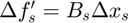
- Smallest weighted Forbenius norm between the current and prior estimate of Hessian (standard BFGS update equation)
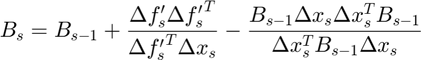 $ Equation (10)
function update_hessian(obj, indx)
%% BFGS initialization:
    gd = find(sum(obj.hist_deltatheta(:,:,indx).^2, 1)>0);% test if there is any history for this subfunction
    num_gd = length(gd);
    %% CASE(I): NO sufficient history to run BFGS
    if num_gd == 0 % if no history, initialize with the median eigenvalue from full Hessian of other subfunctions;
        obj.b(:,:,indx) = 0.;
        H = obj.get_full_H_with_diagonal();
        [U, ~] = obj.eigh_wrapper(H);
        obj.min_eig_sub(indx) = median(U)/sum(obj.active); % median eigenvalue of avg Hessian of other active subfunctions
        obj.max_eig_sub(indx) = obj.min_eig_sub(indx);
        if obj.eval_count(indx) > 2
            if sum(obj.eval_count) < 5 % Subfunction was evaluated multiple times, but has no stored history.
                obj.min_eig_sub(indx) = obj.min_eig_sub(indx) / 10.; % Need to initialize SFO with a smaller hessian_init value >> scale down the hessian_init value
            end
        end
        return;
    end
    %% CASE(II): enough history to run BFGS
    % Working in the subspace defined by this subfunction's history (P_hist);
    [P_hist, ~] = qr([obj.hist_deltatheta(:,gd,indx),obj.hist_deltadf(:,gd,indx)], 0);
    deltatheta_P = P_hist.' * obj.hist_deltatheta(:,gd,indx);
    deltadf_P = P_hist.' * obj.hist_deltadf(:,gd,indx);
    %% approximate the smallest eigenvalue \beta by solving the squared secant equation for full history;
    %% \beta will be used as diagonal initialization for BFGS, (i.e. B_0=\beta I);
    % calculate Hessian using pinv & squared equation:
    % \Delta f_{s}^{'}=B_s \Delta x_s (secant equation >>(df = H dx))
    % (df^T df = dx^T H^T H dx = dx^T H^2 dx)
    % Q=\left [(\Delta x)^{+^{T}} (\Delta f^{'})^{T} \Delta f^{'} (\Delta x)^{+}\right ]^{1/2} Equation (12)
    pdelthet = pinv(deltatheta_P);
    dd = (deltadf_P) * (pdelthet);
    H2 = (dd.') * (dd);
    [H2w, ~] = obj.eigh_wrapper(H2);
    H2w = sqrt(abs(H2w));
    H2w = sort(H2w, 'descend'); % only the top (~num_gd) eigenvalues are expected to be well defined;
    H2w = H2w(1:num_gd);

% Enforcing positive definiteness for the estimated Hessian: Each estimated $ {H_{i}}^t$ is constrained to be +ve definite by explicit eigendecomposition and seeting any
% too-small eigen values to the median positive eigenvalue.
    if min(H2w) == 0 || sum(~isfinite(H2w)) > 0 % ~zero eigenvalue or close (poor estimate of curvature)
    % a failure using this history due to degenerate deltadf (0 case) or deltatheta (non-finite case).;
        H2w(:) = max(obj.min_eig_sub(obj.active)); % Initialize using other subfunctions;
    end
    obj.min_eig_sub(indx) = min(H2w);
    obj.max_eig_sub(indx) = max(H2w);
    % constraining Hessian initialization
    if obj.min_eig_sub(indx) < obj.max_eig_sub(indx)/obj.hess_max_dev % eigenvalues less than (\gamma \lambda_{max})
        obj.min_eig_sub(indx) = obj.max_eig_sub(indx)/obj.hess_max_dev; % constrain using the allowed ratio;
    end

    %% Recalculate Hessian;
    num_hist = size(deltatheta_P, 2); % number of history terms (columns);
    % the new hessian will be (b_p)*(b_p.') + eye().*obj.min_eig_sub(indx);
    b_p = zeros(size(P_hist,2), num_hist*2);
    % step through the history;
    for hist_i = num_hist:-1:1
        s = deltatheta_P(:,hist_i);
        y = deltadf_P(:,hist_i);
        % for numerical stability;
        rscl = sqrt(sum(s.^2));
        s = s/rscl;
        y = y/rscl;
        % the BFGS step proper
        Hs = s.*obj.min_eig_sub(indx) + b_p*((b_p.')*(s));
        term1 = y/sqrt(sum(y.*s));
        sHs = sum(s.*Hs);
        term2 = sqrt(complex(-1.)).*Hs/sqrt(sHs);
        if sum(~isfinite(term1)) > 0 || sum(~isfinite(term2)) > 0
            obj.min_eig_sub(indx) = max(H2w); % invalid bfgs history term
            continue;
        end
        b_p(:,2*(hist_i-1)+2) = term1;
        b_p(:,2*(hist_i-1)+1) = term2;
    end

    H = real((b_p) * (b_p.')) + eye(size(b_p, 1))*obj.min_eig_sub(indx);
    % constrain the Hessian to be positive definite;
    [U, V] = obj.eigh_wrapper(H);
    if max(U) <= 0. %if there aren't any positive eigenvalues after BFGS
        U(:) = obj.max_eig_sub(indx); % set them all to be the same conservative diagonal value;
    end
    % set any too-small eigenvalues to the median positive eigenvalue;
    U_median = median(U(U>0));
    U(U<(max(abs(U))/obj.hess_max_dev)) = U_median;
    % Hessian after it's been forced to be positive definite;
    H_posdef = bsxfun(@times, V, U') * V.';
    % break it apart into matrices b & a diagonal term again;
    B_pos = H_posdef - eye(size(b_p, 1))*obj.min_eig_sub(indx);
    [U, V] = obj.eigh_wrapper(B_pos);
    b_p = bsxfun(@times, V, sqrt(obj.reshape_wrapper(U, [1,-1])));
    obj.b(:,:,indx) = 0.;
    obj.b(:,1:size(b_p,2),indx) = (P_hist)*(b_p);
end
iii. The full approximated Hessian is etimated using the function get_full_H_with_diagonal(obj).
function full_H_combined = get_full_H_with_diagonal(obj)
% Get the full approximate Hessian, including diagonal terms that are included in obj.full_H
    full_H_combined = obj.full_H + eye(obj.K_max).*sum(obj.min_eig_sub(obj.active));
end
3.5 Detecting bad updates
Bad proposed parameter updates are identidied using the function handle_step_failure(obj, f, df_proj, indx). Since only one subfunction is evaluated per update step, a line search on the full objective is impossible, therefore upades are instead lablelled bad when the value of subfunction has increased since its previous evaluation, and also exceeds its approximating function by more than the corresponding reduction in the summed approximating function (i.e.  )
)
When a bad update is detected, is reset to its previous value  , the BFGS history matrices are also updated to include the change in gradient in the failed update direction and the step length is updated as follows
Case 1: successful update 
Case 2: failed update  Equation (16)
function [step_failure, f, df_proj] = handle_step_failure(obj, f, df_proj, indx)
% Check if an update step failed and hence update current position;
    step_failure = false; % check to see whether the step should be a failure;
    if ~isfinite(f) || sum(~isfinite(df_proj))>0
        step_failure = true; % if function or its gradient is not-finite then it's failure;
    elseif obj.eval_count(indx) == 1 % new subfunction with only one evaluation
        if max(obj.eval_count) > 1
            if f > mean(obj.hist_f(obj.eval_count>1,1)) + 3*std(obj.hist_f(obj.eval_count>1,1))
                step_failure = true; % much larger than expected then it's failure;
            end
        end
    elseif f > obj.hist_f(indx,1) % subfunction has increased in value compared to its history
        % (in this case we check if it's larger than its predicted value by enough to trigger a failure);
        f_pred = obj.get_predicted_subf(indx, obj.theta_proj); % calculate the predicted value of this subfunction;
        % subfunction exceeds its predicted value by more than average gain in other subfunctions ?
        predicted_improvement_others = obj.f_predicted_total_improvement - (obj.hist_f(indx,1) - f_pred);
        if f - f_pred > predicted_improvement_others
            step_failure = true; % then the step is failure
        end
    end
    % Step length in both cases (Equation (16))
    if ~step_failure
        obj.step_scale = 1./obj.N + obj.step_scale .* (1. - 1./obj.N); % decay the step_scale back towards 1;
    else
        obj.step_scale = obj.step_scale / 2.; % shorten the step length;
        % subspace may be updated during the function calls so store this in the full space;
        df = (obj.P) * (df_proj);
        [f_lastpos, df_lastpos_proj] = obj.f_df_wrapper(obj.theta_prior_step, indx);
        df_lastpos = (obj.P) * (df_lastpos_proj);

        % if the function value exploded, then back it off until it's a reasonable order of magnitude before adding anything to the history;
        f_pred = obj.get_predicted_subf(indx, obj.theta_proj);
        if isfinite(obj.hist_f(indx,1))
            predicted_f_diff = abs(f_pred - obj.hist_f(indx,1));
        else
            predicted_f_diff = abs(f - f_lastpos);
        end
        if ~isfinite(predicted_f_diff) || predicted_f_diff < obj.eps
            predicted_f_diff = obj.eps;
        end

        for i_ls = 1:10
            if f - f_lastpos < 10*predicted_f_diff % failed update within an order of magnitude of the target update value
                break; % no backoff required;
            end
            % make the step length a factor of 100 shorter;
            obj.theta = 0.99.*obj.theta_prior_step + 0.01.*obj.theta;
            obj.theta_proj = (obj.P.') * (obj.theta);
            % recompute f & df at this new location;
            [f, df_proj] = obj.f_df_wrapper(obj.theta, indx);
            df = (obj.P) * (df_proj);
        end
        % move into the subspace.;
        df_proj = (obj.P.') * (df);
        df_lastpos_proj = (obj.P.') * (df_lastpos);

        if f < f_lastpos % step failed, but last position was even worse (original objective is better);
            theta_lastpos_proj = (obj.P.') * (obj.theta_prior_step);
            obj.update_history(indx, theta_lastpos_proj, f_lastpos, df_lastpos_proj); % add the newly evaluated point to the history;
        else % step failed but proposed f
            % add the change in theta & the change in gradient to the history for this subfunction before failing over to the last position;
            if isfinite(f) && sum(~isfinite(df_proj))==0
                obj.update_history(indx, obj.theta_proj, f, df_proj);
            end
            f = f_lastpos;
            df_proj = df_lastpos_proj;
            obj.theta = obj.theta_prior_step;
            obj.theta_proj = (obj.P.') * (obj.theta);
        end
    end
end
3.6 Growing the number of active subfunctions
The algorithm begins with only small number of active subfunctions (two for our implementation) and expands the active set as learning progresses by one subfunction every time the average gradient shrinks to within a factor  of the standard error in the average gradient, i.e. the active subset is incremented whenever
 Equation (14)
where  is the active subset size at time,
  is the full Hessian, and
  is the average gradient given by:
 Equation (15)
The active subset is also increased when a bad update is detected or when a full pass through the active batch occurs without a batch size increase
function expand_active_subfunctions(obj, full_H_inv, step_failure)
    % expand the set of active subfunctions as appropriate;

    % power in the average gradient direction;
    df_avg = mean(obj.last_df(:,obj.active), 2); % average gradient (Equation (15))
    p_df_avg = sum(df_avg .* (full_H_inv * df_avg)); % part of Equation (14)
    % power of the standard error;
    ldfs = obj.last_df(:,obj.active) - df_avg*ones(1,sum(obj.active));
    num_active = sum(obj.active); % size of the active subset
    p_df_sum = sum(sum(ldfs .* (full_H_inv * ldfs))) / num_active / (num_active - 1);
    % increase size of the active set if standard errror in the estimated gradient is the same order of magnitude as the gradient;
    increase_desirable = (p_df_sum >= p_df_avg.*obj.max_gradient_noise);
    % increase size of the active set on step failure;
    increase_desirable = increase_desirable || step_failure;
    % increase size of the active set if a full pass is done without updating it;
    increase_desirable = increase_desirable || (obj.iter_since_active_growth > num_active);
    % check that all subfunctions have enough evaluations for a Hessian approximation before having new subfunctions;
    eligibile_for_increase = (min(obj.eval_count(obj.active)) >= 2);
    % one more iteration has passed since the active set was last expanded;
    obj.iter_since_active_growth = obj.iter_since_active_growth + 1;
    if increase_desirable && eligibile_for_increase && sum(~obj.active) > 0
        % the index of the new subfunction to activate;
        new_gd = find(~obj.active);
        new_gd = new_gd(randperm(length(new_gd), 1));
        if ~isempty(new_gd)
            obj.iter_since_active_growth = 0;
            obj.active(new_gd) = true;
        end
    end
end
3.7 Perform One Step Optimization
After we defined all these subfunctions, we can perform a single optimization step.
- Choose an index using get_target_index() function.
- Calculate the gradient,
- Calculate inverse of hessian
- Performe finally the Newton step according to Equation (5). (The Newton step length is adjusted in order to avoid numerical errors caused by small numbers or bouncing around opitimized values caused by large step size.)
- Active subfunction set is expended at the end.
 Equation(5)
function optimization_step(obj)
% Perform a single optimization step.
    time_pass_start = tic();
    indx = obj.get_target_index(); %% choose an index to update;
    [f, df_proj] = obj.f_df_wrapper(obj.theta, indx); % evaluate subfunction value & gradient at new position;
    [step_failure, f, df_proj] = obj.handle_step_failure(f, df_proj, indx); % check for a failed update step, & adjust f, df, & obj.theta;
    % as appropriate if one occurs.;
    obj.update_history(indx, obj.theta_proj, f, df_proj); % add the change in theta & the change in gradient to the history for this subfunction;
    obj.total_distance = obj.total_distance + sqrt(sum((obj.theta - obj.theta_prior_step).^2)); % increment the total distance traveled using the last update;
    H_pre_update = real(obj.b(:,:,indx) * obj.b(:,:,indx).'); % the current contribution from this subfunction to the total Hessian approximation;
    obj.update_hessian(indx);%% update this subfunction's Hessian estimate;
    H_new = real(obj.b(:,:,indx) * obj.b(:,:,indx).');% the new contribution from this subfunction to the total approximate hessian;
    obj.full_H = obj.full_H + H_new - H_pre_update;% update total Hessian using this subfunction's updated contribution;

    % calculate the total gradient, total Hessian, & total function value at the current location;
    full_df = 0.;
    for i = 1:obj.N
        dtheta = obj.theta_proj - obj.last_theta(:,i);
        bdtheta = obj.b(:,:,i).' * dtheta;
        Hdtheta = real(obj.b(:,:,i) * bdtheta);
        Hdtheta = Hdtheta + dtheta.*obj.min_eig_sub(i); % the diagonal contribution;
        full_df = full_df + Hdtheta + obj.last_df(:,i);
    end
    full_H_combined = obj.get_full_H_with_diagonal();
    full_H_inv = inv(full_H_combined);
    % calculate an update step;
    dtheta_proj = -(full_H_inv) * (full_df) .* obj.step_scale;% calculate the Newton step described in Equation (5)
    dtheta_proj_length = sqrt(sum(dtheta_proj(:).^2));
    if dtheta_proj_length < obj.minimum_step_length
        dtheta_proj = dtheta_proj*obj.minimum_step_length/dtheta_proj_length;% forcing the update to have minimum step length to avoid numerical errors
        dtheta_proj_length = obj.minimum_step_length;% assign the minimum step length to the update step length
    end
    if sum(obj.eval_count) > obj.N && dtheta_proj_length > obj.eps
    % only allow a step to be up to a factor of max_step_length_ratio longer than the average step length
        avg_length = obj.total_distance / sum(obj.eval_count);
        length_ratio = dtheta_proj_length / avg_length;
        ratio_scale = obj.max_step_length_ratio;
        if length_ratio > ratio_scale
            % truncating step length from (dtheta_proj_length) to (ratio_scale*avg_length)
            dtheta_proj_length = dtheta_proj_length/(length_ratio/ratio_scale);
            dtheta_proj = dtheta_proj/(length_ratio/ratio_scale);
        end
    end

    dtheta = (obj.P) * (dtheta_proj);% the update to theta, in the full dimensional space;
    obj.theta_prior_step = obj.theta;% backup the prior position, in case this is a failed step;
    obj.theta = obj.theta + dtheta;% update theta to the new location;
    obj.theta_proj = obj.theta_proj + dtheta_proj;
    % the predicted improvement from this update step;
    obj.f_predicted_total_improvement = 0.5 .* dtheta_proj.' * (full_H_combined * dtheta_proj);
    obj.expand_active_subfunctions(full_H_inv, step_failure); %% expand the set of active subfunctions as appropriate;
    % record how much time was taken by this learning step;
    time_diff = toc(time_pass_start);
    obj.time_pass = obj.time_pass + time_diff;
end
4. Set Up Hyperparameters
Set Autoencoder structure and training dataset parameters
M = 784; % number visible units
J = 50; % number hidden units
D = 10000; % full data batch size
N = floor(sqrt(D)/10.); % number minibatches
5. Data Import
The dataset we used in this project is MNIST dataset.
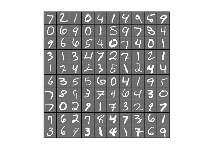
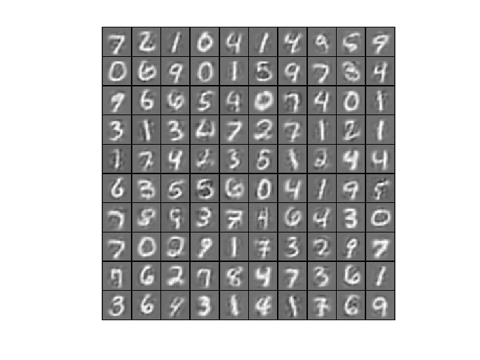
v = loadMNISTImages('train-images-idx3-ubyte.idx3-ubyte');

% create the cell array of subfunction specific arguments
sub_refs = cell(N,1);
for i = 1:N
    % extract a single minibatch of training data.
    sub_refs{i} = v(:,i:N:end);
end

display_network(v(:,1:100));
6. Optimize Autoencoder Using SFO on MNIST Dataset
initialize parameters
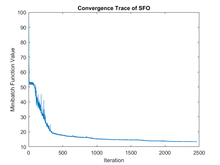
r  = sqrt(6) / sqrt(M+J+1);   % we'll choose weights uniformly from the interval [-r, r]
w = randn(J,M) * 2 * r - r;
b_h = randn(J,1);
b_v = randn(M,1);
b_h = zeros(J,1);
b_v = zeros(M,1);

theta_init = {w, b_h, b_v};
% initialize the optimizer
optimizer = sfo(@f_df_autoencoder, theta_init, sub_refs);
maxIteration = 200;
theta = optimizer.optimize(maxIteration);

% plot the convergence trace
plot(optimizer.hist_f_flat);
xlabel('Iteration');
ylabel('Minibatch Function Value');
title('Convergence Trace of SFO');
6.1 Reconstruction of Autoencoder Trained by SFO
Randomly pick up 100 samples to test the reconstruction performence of trained autoencoder
testSamples = v(:,1:100);
[reconstructed_testSamples] = autoencoder(theta, testSamples);
%Original testSamples
figure(); display_network(testSamples);

%Reconstructed testSamples
figure(); display_network(reconstructed_testSamples);

7. Optimize Autoencoder Using Other Optimizers On MNIST Dataset
Use <http://www.cs.ubc.ca/~schmidtm/Software/ lbfgs> to minimize the same objective function
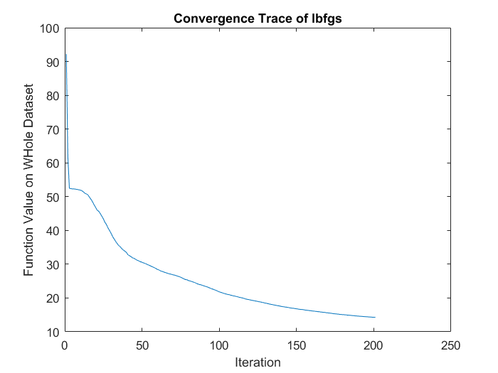
addpath ./minFunc/
options.Method = 'lbfgs'; % Here, we use L-BFGS to optimize our cost
                          % function. Generally, for minFunc to work, you
                          % need a function pointer with two outputs: the
                          % function value and the gradient. In our problem,
                          % sparseAutoencoderCost.m satisfies this.
options.maxIter = 200;	  % Maximum number of iterations of L-BFGS to run
options.display = 'off';

theta_init2 = [w(:) ; b_h(:) ; b_v(:)];

%  Run fminlbfgs
[opttheta, loss, flag, trace] = minFunc( @(p)f_df_autoencoder(p,v), ...
                                        theta_init2, options);

plot(trace.trace.fval);
xlabel('Iteration');
ylabel('Function Value on WHole Dataset');
title('Convergence Trace of lbfgs');
7.1 Reconstruction of Autoencoder Trained by lbfgs
testSamples = v(:,1:100);
[reconstructed_testSamples] = autoencoder(opttheta, testSamples);
%Original testSamples
figure(); display_network(testSamples);
%Reconstructed testSamples
figure(); display_network(reconstructed_testSamples);


8. Analysis and conclusions
Experiment results analysis:
- Comparing convergence traces produced by SFO and lbfgs, we can see that both optimizers converge to a similar optimal function value i.e. around 15. This can also be seen from the reconstruction results that the reconstructed figures of Autoendoers trained by SFO and lbfgs respecitvely look very similar.
- Another obvious character is that the convergence trace produced by SFO is less smooth than the trace produced by lbfgs. This is bacause SFO trains objective function on subfunction i.e. minibatches rather than on a whole dataset as lbfgs does. Although the convergence trance is less smooth, SFO needs less running time memory than lbfgs, and this feature will be more important in task with very large training dataset.
- The way that SFO works on subfunctions of objective function also brings it a disadvantage in task with small dataset.
Summarize Key Features of SFO:
- Single subfunction is evaluated per update step, hence quadratic approximation is maintained for each to get the full hessian estimation (direct target for SFO). Other algorithms considered the hessian of each subfunction as a noisy approximation to the full Hessian.
- Recent history of gradients and positions for each subfunction (iterates) is used to determine a shared and adaptive low dimensional subspace where active subfunctions are stored, manipulated and updated. This guarantees that subspace includes both the steepest gradient descent direction over the full batch as well as update directions from the most recent newton steps. This way SFO algorithm maintains computational tractability and limits memory requirements in the face of high dimensional optimization problems (large M).
- The algorithm initializes the approximate hessian for each subfunction using a diagonal matrix (identity times median eigenvalue of other active subfunctions average hessian (no history), or identity times minimum eigenvalue found by solving squared secant equation (available history)). It might be effective to use the average approximate hessian from all other subfunctions for this initialization that would be overwritten by divergence of individual subfunctions. This way will take the advantage that different subfunctions (for many objective functions) have very similar hessians.
References
[1] Sohl-Dickstein, Jascha, Ben Poole, and Surya Ganguli. "Fast large-scale optimization by unifying stochastic gradient and quasi-newton methods." In International Conference on Machine Learning, pp. 604-612. 2014.
[2] Boyd, Stephen, and Lieven Vandenberghe. Convex optimization. Cambridge university press, 2004.