ECE 602 Project: Modeling the Space of Camera Response Functions
Team members: Si Yan (20711049) and Zhuoran Li (20457147)
Contents
- 1. Background Introduction and Problem Formulation
- 2. Theoretical Space of Camera Response Functions
- 3. Proposed Solution for Camera Response Functions Approximation
- 4.Data Sources
- 5. Solution of the Optimization Problem
- 6. Reproduction of the Simulation Results
- 6.1 Base Function, Basis Vectors and the Energy of Principal Components
- 6.2 EMoR Approximation Performance
- 6.3 Curve Approximation Performance from Sparse Samples
- 6.4 Evaluation of the Performance of the EMoR Model as the Number of Parameters Increase
- 6.5 Performance Comparison with traditional Curve Approximation Methods
- 7. Conclusions
- 8. Reference
1. Background Introduction and Problem Formulation
Computer vision applications have been greatly developed and used in the recent years. The model of a certain imaging system which can describe the relationship between the scene radiance and the image intensity plays an important role in designing the computer vision algorithms[1].
Typically, an imaging system first transform the scene radiance to the image irradiance, and then the irradiance value will be mapped to the image intensity. This mapping function is called camera response function which is nonlinear. In this paper, authors proposed a curve approximation method to estimate the camera response function based on the limited information of the function. The theoretical analysis demonstrated that all the response functions are inside a convex set. The proposed estimation algorithm was evaluated by a set of real-world camera response functions.
2. Theoretical Space of Camera Response Functions
The model of the space of camera response functions are formulated based on the following assumptions:
- One response function is applied to all the pixels of a certain image;
- The value of each image irradiance (
 ) is normalized. In other words,
 ![$\forall E \in [0, 1]$](main_eq06641582333971295590.png) ;
; - All the response functions are normalized and monotonic. Hence, the value of image intensity (
 ) belongs to
 ![$[0, 1]$](main_eq03339228126667836648.png) .
.
The space of the camera response functions are defined as:
 .
.
It is shown in [1] that  is the intersection of a convex cone and a hyperplane. Therefore, the function space is a convex set. Any positive linear combination of the response functions is also a response function.
3. Proposed Solution for Camera Response Functions Approximation
- General Curve Approximation Model
Since the response functions in theoretical space have infinite dimensions, they cannot be implemented in practice. In this paper, authors first utilized a general curve approximation method with finite parameters which is expressed as following:
 ,
,
where  is a chosen base response function.
  are the basis of the vector space with
  . In addition, the optimization variables
  are the weights to be determined to minimize the curve estimation error.
- Empirical Model of Reponse (EMoR)
In this paper, authors used the response curves which collected from real-world imaging systems to determine the appropriate basis vectors and the base response function. The dataset contains 201 measured curves which are divided into a training set and a testing set. The training set and the testing set have 175 and 26 curves, respectively.
As we discussed before, the space of the camera response functions () is a convex cone. Therefore, the base function ( ) is selected as the mean of all the response curves in the training set which is described as
 ,
,
where  .
.  denotes the
  curve in the training set. The Principal Component Analysis (PCA) is used to compute the basis vectors. The basis vectors are the eigenvectors of the covariance matrix of the training curves. The covariance matrix is expressed as

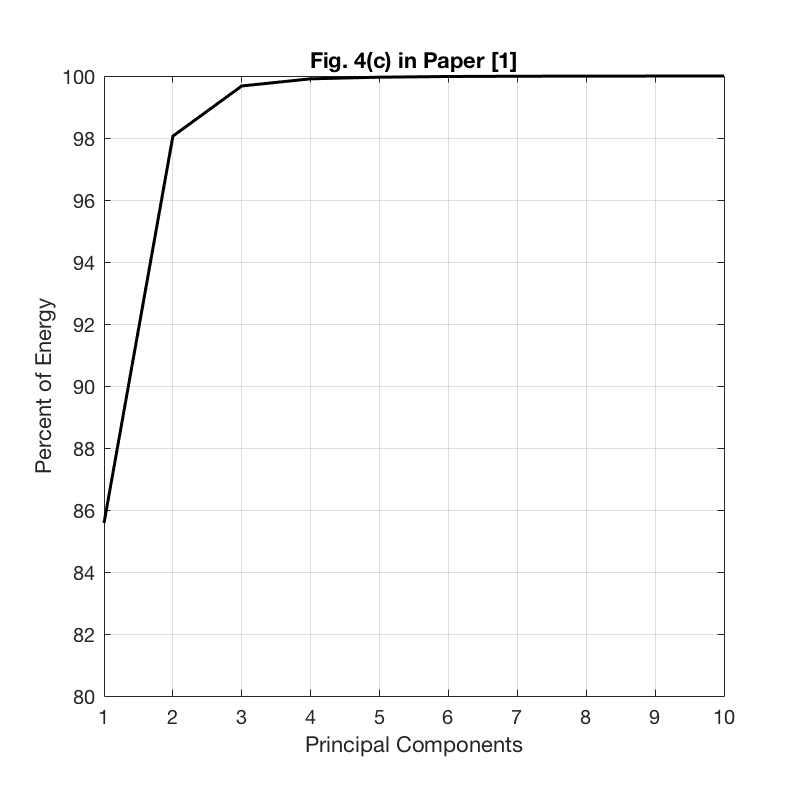
Considering we need  basis vectors to approximate the response function. The eigenvectors of the largest eigenvalues are selected as the basis. The authors showed that 3 largest eigenvalues contains more than 99$%$ of the energy. Hence, we can use low-dimensional data estimate the response function.
- Mathematical Expression of the Optimization Problem
After we determine the base curve and the basis vectors, we only need to calculate the parameters . This process is formulated as an optimization problem that is described as following:

 represents the basis matrix and
  is the derivative matrix. The constraint indicates that all the camera response functions should be monotonically increasing. Therefore, their derivatives are all positive values. Note that, parameters are the optimization variables .
- Response Function Approximation From Sparse Samples
In this paper, authors also demonstrated that EMoR can estimate the response functions more accurate than other algorithms from the sparse samples of the original camera response functions.
4.Data Sources
In this paper, all the response functions from training set and testing set are measured from real-world imaging systems. The dataset can be downloaded from http://www.cs.columbia.edu/CAVE .
5. Solution of the Optimization Problem
The optimization problem discussed in section 3 is a quadratic programming problem which can be solved by MATLAB CVX toolbox. In addition, The convexity of the response function space indicates that there is a unique optimum solution.
6. Reproduction of the Simulation Results
In this section, we will reproduce the simulation results from [1] by using the MATLAB CVX toolbox. Note that , Figure 1,2,3,5,6 are utilized to support the paper description which are not included in this section.
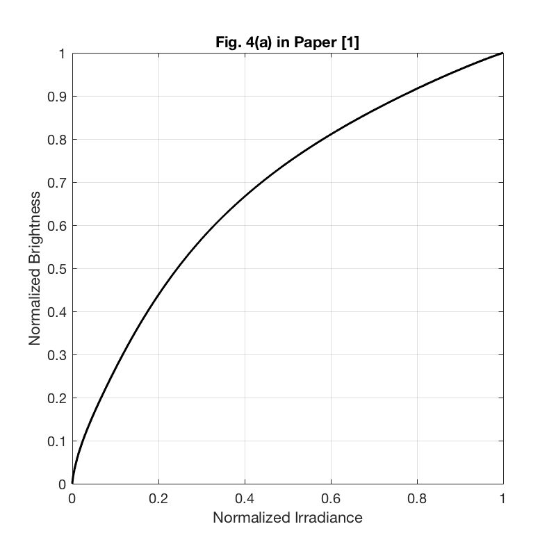
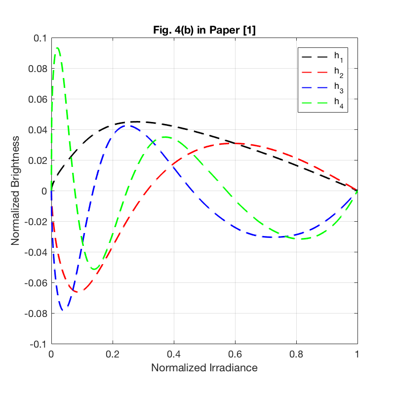
6.1 Base Function, Basis Vectors and the Energy of Principal Components
clear all
close all

% Loading dataset
formatSpec = '%f';
trainFile = fopen('dataTrain.txt', 'r'); % training data
testFile = fopen('dataTest.txt', 'r'); % testing data
irradianceFile = fopen('dataI.txt', 'r'); % irradiance data

trainSet1 = fscanf(trainFile, formatSpec);
testSet1 = fscanf(testFile, formatSpec);
irradianceSet1 = fscanf(irradianceFile, formatSpec);

fclose(trainFile);
fclose(testFile);
fclose(irradianceFile);

[s_tr, col] = size(trainSet1); % size of traning set
[s_te, col] = size(testSet1); % size of testing set
[s_irr, col] = size(irradianceSet1); % size of irradiance set

train_data_num = s_tr/1024; % number of training curves
test_data_num = s_te/1024; % number of testing curves

train_set = reshape(trainSet1, [1024, train_data_num])'; % 175 training samples
test_set = reshape(testSet1, [1024, test_data_num])'; % 26 testing samples
irradiance_set = irradianceSet1;

% Base function
f0 = zeros(1,1024);
f0_log = zeros(1,1024);

for i = 1:1024
    % base function is the average over all the response curves in the
    % training set
    f0(i) = sum(train_set(:,i))/175;
end

for i = 1:1024
    f0_log(i) = geo_mean(train_set(:,i)); % base function in the log-space
end

for i = 1:train_data_num
    train_set(i, :) = train_set(i, :) - f0;
end

cov_matrix = cov(train_set); % the covariance matrix of the training curves

eig_values = eig(cov_matrix); % calculate the eigenvalues of the covariance matrix
[eig_vectors, D] = eig(cov_matrix); % calculate the eigenvectors of the covariance matrix, each column of eig_vectors is an eigenvector

eig_values1 = real(eig_values);
eig_vectors1 = real(eig_vectors);

for i = 1:1024
    eig_values(i) = eig_values1(1024-i+1); % sort the eigenvalues
end

for i = 1:1024
    eig_vectors(:, i) = eig_vectors1(:, 1024-i+1); % sort the eigenvectors
end

num_principals = 25; % number of the principal components used in curve approximation

principals = eig_vectors(:, 1:num_principals); % the largest 25 eigenvalues are the principal components

principal_energy = zeros(1, num_principals);

for i = 1:num_principals
    principal_energy(i) = sum(eig_values(1:i))/sum(eig_values); % energy percentage of the principal components
end

% Plot Figure 4 in [1]
figure();
set(gcf, 'position', [100 100 400 400]);
plot(irradiance_set, f0, 'k','LineWidth', 1.5); % plot the base function f0
grid on
xlabel('Normalized Irradiance')
ylabel('Normalized Brightness')
title('Fig. 4(a) in Paper [1]');
axis square

figure();
set(gcf, 'position', [100 100 400 400]);
plot(irradiance_set, principals(:,1), '--k', 'LineWidth', 1); % plot the largest 4 basis vectors
hold on
plot(irradiance_set, principals(:,2), '--r', 'LineWidth', 1);
hold on
plot(irradiance_set, principals(:,3), '--b', 'LineWidth', 1);
hold on
plot(irradiance_set, principals(:,4), '--g', 'LineWidth', 1);
hold off
grid on
legend('h_{1}', 'h_{2}', 'h_{3}', 'h_{4}');
xlabel('Normalized Irradiance')
ylabel('Normalized Brightness')
title('Fig. 4(b) in Paper [1]');
axis([0 1 -0.1 0.1]);
axis square

figure();
set(gcf, 'position', [100 100 400 400]);
plot([1:10], principal_energy(1:10)*100, 'k', 'LineWidth', 1.5); % plot the energy function
grid on
xlabel('Principal Components')
ylabel('Percent of Energy')
title('Fig. 4(c) in Paper [1]');
axis([1 10 80 100]);
axis square
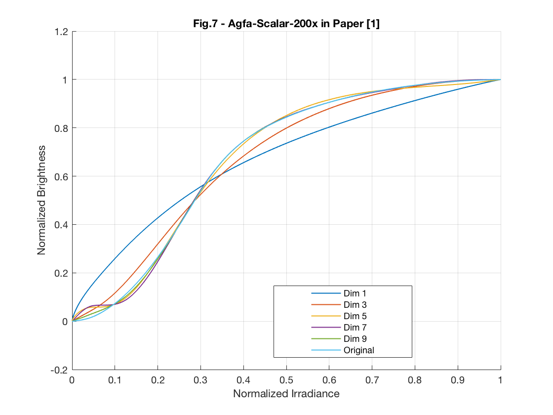
6.2 EMoR Approximation Performance
In this part, we plot the Figure 7 in [1] which indicates the relationship between the estimation performance and the number of principal components.
for i = 1:train_data_num
    train_set(i, :) = train_set(i, :) + f0;
end

test_vector_index = 170; % Index of gamma curve, g=2.4
test_vector = train_set(test_vector_index, :); % testing response curve

sample_point_index = [100, 250, 400, 550, 700, 850];

test_sample_points = test_vector(sample_point_index); % sparse samples from the testing curve
f0_sample_points = f0(sample_point_index); % sparse samples from the base function

v = test_sample_points - f0_sample_points;

D = zeros(1023, 1024); % derivative matrix

for i = 1:1023
    D(i, i) = -1./(irradiance_set(i+1) - irradiance_set(i));
    D(i, i+1) = 1./(irradiance_set(i+1) - irradiance_set(i));
end

figure();
hold all
for num_principals = [1 3 5 7 9]
    principals = eig_vectors(:, 1:num_principals);
    principals_sample_points = principals(sample_point_index, :); % sparse samples from the principal components

    % solving quadratic programming problem by CVX
    cvx_begin quiet
        variable c(num_principals) % optimization variables

        minimize( norm( principals_sample_points*c - v' , 2) ) % objective function

        (-1)*D*principals*c - D*f0' <= 0 % constraint: all response functions are monotonically increasing
    cvx_end

    f_approx_mon = principals * c + f0'; % approximation of the testing response curve

    plot(irradiance_set, f_approx_mon, 'LineWidth', 1);
end
plot(irradiance_set, test_vector, 'LineWidth', 1);
hold off;
grid on
gca = legend('Dim 1', 'Dim 3', 'Dim 5', 'Dim 7', 'Dim 9', 'Original');
set( gca, 'Position', [0.495 0.14 0.25 0.17]);
xlabel('Normalized Irradiance')
ylabel('Normalized Brightness')
axis([0 1 -0.2 1.2]);
title('Fig.7 - Gamma Curve, g=2.4 in Paper [1]')

test_vector_index = 59; % Index of agfa-scalar-200x
test_vector = train_set(test_vector_index, :); % testing response curve

sample_point_index = [100, 250, 400, 550, 700, 850];

test_sample_points = test_vector(sample_point_index); % sparse samples from the testing curve
f0_sample_points = f0(sample_point_index); % sparse samples from the base function

v = test_sample_points - f0_sample_points;

D = zeros(1023, 1024); % derivative matrix

for i = 1:1023
    D(i, i) = -1./(irradiance_set(i+1) - irradiance_set(i));
    D(i, i+1) = 1./(irradiance_set(i+1) - irradiance_set(i));
end

figure();
hold all
for num_principals = [1 3 5 7 9]
    principals = eig_vectors(:, 1:num_principals);
    principals_sample_points = principals(sample_point_index, :); % sparse samples from the principal components

    % solving quadratic programming problem by CVX
    cvx_begin quiet
        variable c(num_principals) % optimization variables

        minimize( norm( principals_sample_points*c - v' , 2) ) % objective function

        (-1)*D*principals*c - D*f0' <= 0 % constraint: all response functions are monotonically increasing
    cvx_end

    f_approx_mon = principals * c + f0'; % approximation of the testing response curve

    plot(irradiance_set, f_approx_mon, 'LineWidth', 1);
end
plot(irradiance_set, test_vector, 'LineWidth', 1);
hold off;
grid on
gca = legend('Dim 1', 'Dim 3', 'Dim 5', 'Dim 7', 'Dim 9', 'Original');
set( gca, 'Position', [0.495 0.14 0.25 0.17]);
xlabel('Normalized Irradiance')
ylabel('Normalized Brightness')
axis([0 1 -0.2 1.2]);
title('Fig.7 - Agfa-Scalar-200x in Paper [1]')

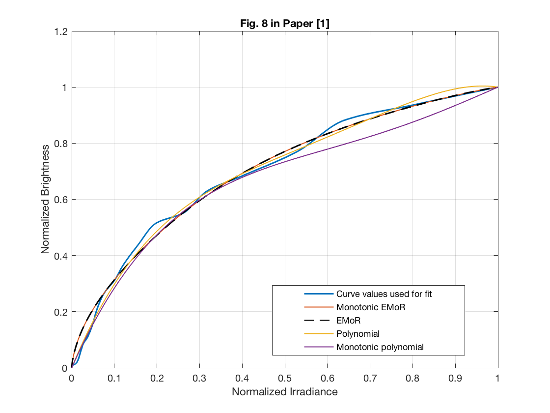
6.3 Curve Approximation Performance from Sparse Samples
In this section, we will reproduce the Figure 8 in [1]. Since the experimental data in this part is not available, we used another response function in the testing set. Therefore, this may cause the simulation results have slightly different curve with the original Figure 8.
test_vector_index = 26;
test_vector = test_set(test_vector_index, :);

sample_point_index = [100, 250, 400, 550, 700, 850];

test_sample_points = test_vector(sample_point_index);
f0_sample_points = f0(sample_point_index);

v = test_sample_points - f0_sample_points;

D = zeros(1023, 1024);

for i = 1:1023
    D(i, i) = -1./(irradiance_set(i+1) - irradiance_set(i));
    D(i, i+1) = 1./(irradiance_set(i+1) - irradiance_set(i));
end

num_principals_sparse = 3;

principals_sparse = eig_vectors(:, 1:num_principals_sparse);
principals_sample_points_sparse = principals_sparse(sample_point_index, :);

% monotonic EMoR curve approximation
cvx_begin quiet
    variable c(num_principals_sparse)
    minimize( norm( principals_sample_points_sparse*c - v' , 2) )
    (-1)*D*principals_sparse*c - D*f0' <= 0
cvx_end

% pure EMoR curve approximation
cvx_begin quiet
    variable c1(num_principals_sparse)
    minimize( norm( principals_sample_points_sparse*c1 - v' , 2) )
cvx_end

f0_poly = irradiance_set';
v_poly = test_sample_points - f0_poly(sample_point_index);
H_poly = zeros(1024,num_principals_sparse);

for i = 1:num_principals_sparse
    H_poly(:,i) = (irradiance_set.^(i+1))' - irradiance_set';
end

H_poly_sample_points = H_poly(sample_point_index, :);

% monotonic polynomial curve approximation
cvx_begin quiet
    variable p(num_principals_sparse)
    minimize( norm( H_poly_sample_points*p - v_poly' , 2) )
    (-1)*D*H_poly*p - D*f0' <= 0
cvx_end

% pure polynomial curve approximation
cvx_begin quiet
    variable p1(num_principals_sparse)
    minimize( norm( H_poly_sample_points*p1 - v_poly' , 2) )
cvx_end

% estimated reponse curves
f_appro_sparse_emor_monoto = principals_sparse * c + f0';
f_appro_sparse_emor = principals_sparse * c1 + f0';

f_appro_sparse_poly_monoto = H_poly * p + f0_poly';
f_appro_sparse_poly = H_poly * p1 + f0_poly';


figure();
plot(irradiance_set, test_vector, 'linewidth', 1.5);
hold on
plot(irradiance_set, f_appro_sparse_emor_monoto, 'linewidth', 1);
hold on
plot(irradiance_set, f_appro_sparse_emor, '--k', 'linewidth', 1);
hold on
plot(irradiance_set, f_appro_sparse_poly, 'linewidth', 1);
hold on
plot(irradiance_set, f_appro_sparse_poly_monoto, 'linewidth', 1);
hold off
grid on
gca = legend('Curve values used for fit', 'Monotonic EMoR', 'EMoR', 'Polynomial', 'Monotonic polynomial');
set( gca, 'Position', [0.495 0.14 0.35 0.17]);
xlabel('Normalized Irradiance')
ylabel('Normalized Brightness')
axis([0 1 0 1.2]);
title('Fig. 8 in Paper [1]')
%
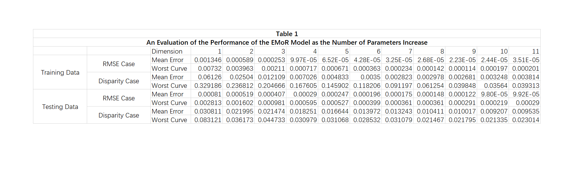
6.4 Evaluation of the Performance of the EMoR Model as the Number of Parameters Increase
In this section, we will reproduce the Table 1 in [1]. Since the exact 175 training response functions in this part is not known, we used the first 175 out of 201 response functions as training set and the rest 26 as testing set. Therefore, this may cause the simulation results have slightly different curve with the original Table 1.
rmse = zeros(175, 11);
disparity = zeros(175, 11);
sample_point_index = 1:30:1024;

D = zeros(1023, 1024);

for i = 1:1023
    D(i, i) = -1./(irradiance_set(i+1) - irradiance_set(i));
    D(i, i+1) = 1./(irradiance_set(i+1) - irradiance_set(i));
end
f0_sample_points = f0(sample_point_index);

for test_vector_index = 1:175
    test_vector = train_set(test_vector_index, :);

    test_sample_points = test_vector(sample_point_index);

    v = test_sample_points - f0_sample_points;

    for num_principals = 1:11
        principals = eig_vectors(:, 1:num_principals);
        principals_sample_points = principals(sample_point_index, :);

        cvx_begin quiet
            variable c(num_principals)

            minimize( norm( principals_sample_points*c - v' , 2) )

            (-1)*D*principals*c - D*f0' <= 0
        cvx_end

        f_approx_mon = principals * c + f0';
        rmse(test_vector_index, num_principals) = ...
            norm(test_vector' - f_approx_mon, 2)/1024;
        disparity(test_vector_index, num_principals) = ...
            max(test_vector' - f_approx_mon);
    end
end
train_rmse_mean = mean(rmse);
train_rmse_worst = max(rmse);
train_disparity_mean = mean(disparity);
train_disparity_max = max(disparity);

rmse = zeros(26, 11);
disparity = zeros(26, 11);
sample_point_index = 1:30:1024;

D = zeros(1023, 1024);

for i = 1:1023
    D(i, i) = -1./(irradiance_set(i+1) - irradiance_set(i));
    D(i, i+1) = 1./(irradiance_set(i+1) - irradiance_set(i));
end
f0_sample_points = f0(sample_point_index);

for test_vector_index = 1:26
    test_vector = test_set(test_vector_index, :);

    test_sample_points = test_vector(sample_point_index);

    v = test_sample_points - f0_sample_points;

    for num_principals = 1:11
        principals = eig_vectors(:, 1:num_principals);
        principals_sample_points = principals(sample_point_index, :);

        cvx_begin quiet
            variable c(num_principals)

            minimize( norm( principals_sample_points*c - v' , 2) )

            (-1)*D*principals*c - D*f0' <= 0
        cvx_end

        f_approx_mon = principals * c + f0';
        rmse(test_vector_index, num_principals) = ...
            norm(test_vector' - f_approx_mon, 2)/1024;
        disparity(test_vector_index, num_principals) = ...
            max(test_vector' - f_approx_mon);
    end
end
test_rmse_mean = mean(rmse);
test_rmse_worst = max(rmse);
test_disparity_mean = mean(disparity);
test_disparity_max = max(disparity);

figure();
table1 = imread('Table1.png');
imshow(table1);
%
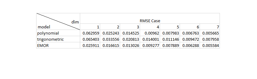
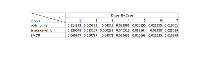
6.5 Performance Comparison with traditional Curve Approximation Methods
In this part, we reproduced the Table 2 and the Table 3 in [1]. Since the authors do not specify the experimental details, we selected 35 samples to approximate the response curves. The reproduced simulation results show that EMoR can achieve better estimation performance than the Polynomial model and the trigonometric model.
RMSE = zeros(3,7);
RMSE_avg = zeros(3,7);
Disparity = zeros(3,7);
Disparity_avg = zeros(3,7);

for w = 1:26

    test_vector_index = w;
    test_vector = test_set(test_vector_index, :);

    for j = 1:7

        sample_point_index = 1:30:1024; % select 35 samples to estimate the response curves

        test_sample_points = test_vector(sample_point_index);
        f0_sample_points = f0(sample_point_index);

        v = test_sample_points - f0_sample_points;

        D = zeros(1023, 1024);

        for i = 1:1023
            D(i, i) = -1./(irradiance_set(i+1) - irradiance_set(i));
            D(i, i+1) = 1./(irradiance_set(i+1) - irradiance_set(i));
        end

        num_principals_sparse = j;

        principals_sparse = eig_vectors(:, 1:num_principals_sparse);
        principals_sample_points_sparse = principals_sparse(sample_point_index, :);

        % EMoR curve approximation
        cvx_begin quiet
            variable c(num_principals_sparse)
            minimize( norm( principals_sample_points_sparse*c - v' , 2) )
            (-1)*D*principals_sparse*c - D*f0' <= 0
        cvx_end

        f0_poly = irradiance_set';
        v_poly = test_sample_points - f0_poly(sample_point_index);
        H_poly = zeros(1024,num_principals_sparse);

        for i = 1:num_principals_sparse
            H_poly(:,i) = (irradiance_set.^(i+1))' - irradiance_set';
        end

        H_poly_sample_points = H_poly(sample_point_index, :);

        % polynomial curve approximation
        cvx_begin quiet
            variable p(num_principals_sparse)
            minimize( norm( H_poly_sample_points*p - v_poly' , 2) )
        cvx_end

        f0_trigonometric = irradiance_set';
        v_trigonometric = test_sample_points - f0_trigonometric(sample_point_index);
        H_trigonometric = zeros(1024,num_principals_sparse);

        for i = 1:num_principals_sparse
            for ii = 1:1024
                H_trigonometric(ii,i) = sin(i*pi*irradiance_set(ii));
            end
        end

        H_trigonometric_sample_points = H_trigonometric(sample_point_index, :);

        % trigonometric curve approximation
        cvx_begin quiet
            variable t(num_principals_sparse)
            minimize( norm( H_trigonometric_sample_points*t - v_trigonometric' , 2) )
        cvx_end

        f_appro_sparse_emor_table = principals_sparse * c + f0';
        f_appro_sparse_poly_table = H_poly * p + f0_poly';
        f_appro_sparse_trigonometric_table = H_trigonometric * t + f0_trigonometric';

        RMSE(1,j) = sqrt(mean((f_appro_sparse_poly_table-test_vector').^2)); % RMSE for Polynomial approximation
        RMSE(2,j) = sqrt(mean((f_appro_sparse_trigonometric_table-test_vector').^2)); % RMSE for trigonometric approximation
        RMSE(3,j) = sqrt(mean((f_appro_sparse_emor_table-test_vector').^2)); % RMSE for ERoR approximation

        Disparity(1,j) = max(abs(f_appro_sparse_poly_table-test_vector')); % disparity for Polynomial approximation
        Disparity(2,j) = max(abs(f_appro_sparse_trigonometric_table-test_vector')); % disparity for trigonometric approximation
        Disparity(3,j) = max(abs(f_appro_sparse_emor_table-test_vector')); % disparity for ERoR approximation
    end

    RMSE_avg = RMSE_avg + RMSE;
    Disparity_avg = Disparity_avg + Disparity;
end

RMSE_avg = (1/26)*RMSE_avg; % Average RMSE for all the testing curves
Disparity_avg = (1/26)*Disparity_avg; % Average Disparity for all the testing curves

figure();
table2 = imread('Table2.png');
imshow(table2);
figure();
table3 = imread('Table3.png');
imshow(table3);
%
7. Conclusions
In this papaer, authors proposed a novel method for estimating the camera reponse curve which combines the general curve approximation algorithm and the empirical approach. The curve esimation process was formulated as a quadratic programming problem. The convex domain implies that there is a unique optimum solution.The model was evaluated by a dataset of real-world imaging systems. The simulation results show that the proposed approximation method can achieve higher estimation accuracy than the traditional models (gamma approximation, polynomial approximation and trigonometric approximation).
In this project, we reproduced the main results from [1]. The reproduced results have similar performance with the original experimental results. Based on the simulation results, we can also have the following observations:
- There is a typo in the optimization problem expression. The objective function should be .
- The curve approximating performance highly depends on the measurement accuracy of the real-world imaging systems. Therefore, the measurement error of the response curves in the training set can greatly degrade the algorithm performance.
- The EMoR model is proposed based a fundamental assumption that all the pixels in an image have the same response function. However, this assumption can not be satisfied in many imaging systems, such as CCD camera.
8. Reference
[1]. M. D. Grossberg and S. K. Nayar, "Modeling the space of camera response functions," IEEE transactions on pattern analysis and machine intelligence, vol. 26, no. 10, pp. 1272-1282, 2004.