ECE 602 - Winter 2018 - Course Project
Topic: Faster and better: A machine learning approach to corner detection [1]
Team member's student ID: 20705349
Contents
Problem Formulation
This is a MATLAB implmentation of the algorithm of corner detection based on the paper "Faster and better: A machine learning approach to corner detection" [1].
Traditional corner detection algorithms usually suffer from the problem of low efficiency particularly in the case of large images. Yet corner detection algorithms play a fundamental role in many image processing algorithms. As such, it is of practical needs to develop a faster corner algorithm. In this paper[1], the author proposed a machine learning based algorithm to detect the corners in an image that has the advantage in terms of speed and accuracy. In the paper, the author proposed that to determine whether a pixel on an image represents a corner, one needs to check the values of its 16 neighboring pixels with respect to the value of the pixel itself.
Therefore, this problem can be essentially formulated as an optimization problem of decision tree.
Proposed Solution
In a given training/testing image, for each pixel of the image  , we need to assign a category to each of its 16 neighboring pixels
  where
where  by deciding whether the neighboring pixel is brighter than, similar to, or darker than the center pixel .
In this way, we can generate a feature vector  for each whose element
  , where
  takes a value from
  depending on
  's relation with .
If  , then
  , if
, if  , then
  and if
  then
then  , where
  is the threshold.
Furthermore, we can extend  to have an additional column
  that takes on a binary value to indicate whether is a corner or not.
Upon extracting the features for all pixels of a given image, we obtain a feature matrix  where each row is the for each pixel of the image.
So we denote the training set  where
where  is the number of pixels in the image.
Suppose  denotes a vector containing the indices of the feature. Then
 ![$x = [1,2,\cdots, 16]$](main_eq05747833932026736134.png) . Among all features, we need to find one that maximizes the information gain
. Among all features, we need to find one that maximizes the information gain
where is the training set. For each  , we could compute its information gain by partitioning these rows into three different groups
  ,
,  , and
, and  based on the value of the column, which could allow the computation of the information gain for by

where  denotes the entropy of the group Q and can be computed via

where  and
and  denote the number of corners and non-corners respectively in group Q.
The  will be used to create the tree's root vertex which has up to three child nodes that are created by recursively running the above algorithm until it converges.
where  , meaning that
  is the original except where is removed from the vector.
This algorithm continues to recursively generate the decision tree nodes based on the ID3 decision tree algorithm until the entropy of becomes zero or when is empty, at which point the tree node will be assigned a binary value that is the mode of the last column of .
Data Sources
We followed the paper [1] and [2] in terms of the use of training and testing images. However, it is important to note that the actual labeled training and testing datasets are not available. In other words, although the images are available, the pixels on these images are not labeled to be corners or non-corners at all. This thus requires our own manual labelings to generate the training and testing datasets. The manual labeling function is included in the support files (labeling.m).
There are a total of 14 images available in the "Box" dataset used in the paper [1,2]. We chose the first 11 to be the training dataset and the rest as testing dataset. On each image, we manually labeled 50 points that appeared to be corners and their indices on the image were recorded. The rest of the pixels on the images were regarded as non-corners.
Solution and Visualization of Results
The threshold needs to be manually chosen and is usually taken in a way that maximizes the overall performance. In this project, was chosen to be  . While this choice may differ from the actual threshold suggested in the paper, one also needs to note that the training dataset the paper originally used was not available and as such, the threshold was not necessarily chosen exactly the same as in the paper [1].
Setting the threshold for and regenerating the training dataset P
clear;close all;clc;
thresh =18;
% generating the training dataset P
tic;
P = gen_features_all('train',thresh);
disp(['Time cost for generating training dataset: ' num2str(toc)]);
The number of images in training datasets: 11...
Generating features P from frame_0.png ...
Generating features P from frame_1.png ...
Generating features P from frame_10.png ...
Generating features P from frame_2.png ...
Generating features P from frame_3.png ...
Generating features P from frame_4.png ...
Generating features P from frame_5.png ...
Generating features P from frame_6.png ...
Generating features P from frame_7.png ...
Generating features P from frame_8.png ...
Generating features P from frame_9.png ...
Feature extraction complete ...
Time cost for generating training dataset: 8.0291
training the decision tree
tic;
disp('training the decision tree ...');
trained_tree = train_decision_tree(P);
training the decision tree ...
displaying the time cost when training is complete
disp(['Time cost for the training process: ' num2str(toc)]);
%load('trained_tree.mat');
Time cost for the training process: 153.8381
Test the tree on a training example to see if the algorithm converges well
file_ = 'frame_5';
test_file = ['./train/' file_ '.png'];
test_corners_file = ['./train_corners/train_' file_ '_corners.mat'];
image_test1(trained_tree, thresh, test_file, test_corners_file);
Testing image ./train/frame_5.png ...
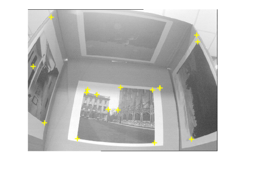
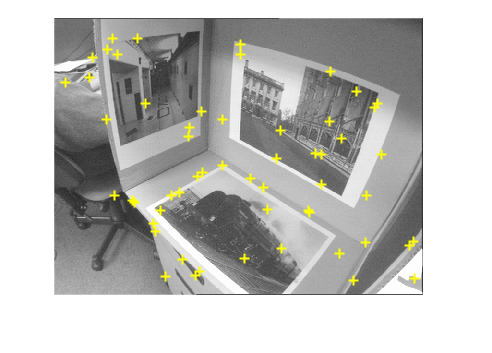
Test the tree on a testing example to see if the algorithm generalizes well
file_ = 'frame_11';
test_file = ['./test/' file_ '.png'];
test_corners_file = ['./test_corners/test_' file_ '_corners.mat'];
image_test1(trained_tree, thresh, test_file, test_corners_file);
Testing image ./test/frame_11.png ...
Test the tree on a MATLAB built-in images to see if the algorithm generalizes well
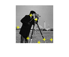
image_test2(trained_tree, 'cameraman.tif', thresh);
Testing image cameraman.tif ...
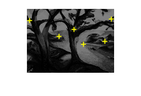
Test the tree on a MATLAB built-in images to see if the algorithm generalizes well
image_test2(trained_tree, 'trees.tif', thresh);
Testing image trees.tif ...
Function that takes the training dataset P and trains the decision tree
function tree = train_decision_tree(P)
    selected_attributes = 1:16;
    tree = decision_tree(P, selected_attributes);
end
Function that recursively generates the decision tree
function tree_node = decision_tree(train, selected_attributes)
tree_node = struct('val',[],'left',[],'mid',[],'right',[]);
if isempty(train)
    return;
end

if compute_entropy(train) == 0 || isempty(selected_attributes)
    tree_node.val = mode(train(:,end));
    return;
end
optimal_x = arg_max_info_gains(train,selected_attributes);
[Pd, Ps, Pb] = partition_into_groups(train, optimal_x);
index_of_optimal_x = find(selected_attributes == optimal_x);
selected_attributes(index_of_optimal_x) = [];

tree_node.val   =  optimal_x;
tree_node.left  =  decision_tree(Pd, selected_attributes);
tree_node.mid   =  decision_tree(Ps, selected_attributes);
tree_node.right =  decision_tree(Pb, selected_attributes);
end
Function that partitions P into three groups by column x of P
function [Pd,Ps,Pb] = partition_into_groups(P, x)
x_column = P(:,x);
indices_of_Pd = find(x_column == 0);
indices_of_Ps = find(x_column == 1);
indices_of_Pb = find(x_column == 2);

Pd = P(indices_of_Pd,:);
Ps = P(indices_of_Ps,:);
Pb = P(indices_of_Pb,:);
end
Function that finds the optimal x that maximizes the information gain
function x = arg_max_info_gains(train, selected_attributes)
num_of_attrs = length(selected_attributes);
if num_of_attrs == 0
    x = [];
    return;
end
if num_of_attrs == 1
    x = selected_attributes;
    return;
end

info_gains = zeros(1, num_of_attrs);
for i = 1:num_of_attrs
    current_x = selected_attributes(i);
    info_gains(i) = compute_info_gain(train, current_x);
end
x = selected_attributes(find(info_gains == max(info_gains)));
x = x(1);% in case there is more than 1 maximum.
end
Function that computes the information gain with respect to x
function gain = compute_info_gain(P, x)
[Pd, Ps, Pb] = partition_into_groups(P, x);
gain = compute_entropy(P) - compute_entropy(Pd) - compute_entropy(Ps) - compute_entropy(Pb);
end
Function that computes the entropy of a set Q
function entropy = compute_entropy(Q)
last_column_of_Q = Q(:,end);
num_of_totals  = length(last_column_of_Q);
num_of_corners = length(find(last_column_of_Q==1));
num_of_non_corners = num_of_totals - num_of_corners;
entropy_total = 0;
entropy_corners = 0;
entropy_non_corners = 0;

if num_of_totals ~= 0
    entropy_total = (num_of_totals) * log2(num_of_totals);
end

if num_of_corners ~= 0
    entropy_corners = num_of_corners*log2(num_of_corners);
end

if num_of_non_corners ~= 0
    entropy_non_corners = num_of_non_corners*log2(num_of_non_corners);
end

entropy =  entropy_total - entropy_corners - entropy_non_corners;
end
Analysis and Conclusions
This implementation has successfully realized the machine learning based algorithm for classifying the corners on a given image.
This implemented algorithm behaves predictably in the sense that it is able to mark some of the corners on an image.
However, from the above testing results, we could also see that the algorithm achieved better performances on the training examples rather than the testing examples. The lack of generalization of the algorithm is primarily due to the absence of the original training dataset that the paper was using. As such, for this project, we had to manually label the training dataset which were of limited amount which could lead to overfitting.
From the experiments, it was clear that the algorithm did perform quite fast upon the completion of the training process, although the training process could take a very long time. Since the original training dataset was not available, it was not possible to fully repeat the experiments as reported in the paper.
The inavailability of the original training dataset used in the paper [1] could entail some drawbacks. For instance, besides 50 pixels labeled as corners on each image, the vast amount of the rest pixles were therefore labeled as non-corners. For this reason, the amount of non-corner examples is much larger than the corner examples which could lead to overfitting. Futhermore, the labeled 50 pixels may not be comprehensive and causing some actual corners to be labeled as non-corners, which could then bring a high level of noise into the training dataset.
Nevertheless, in this project, we have successfully implemented the machine learning based algorithm for corner detection as introduced in the paper [1] and tested it on a number of testing images.
List of Necessary Files/Functions for the Implementation
The following is a list of the necessary functions
classify_corners.m
image_features.m
gen_features_all.m
image_test1.m
image_test2.m
labeling.m
References
[1] Rosten, E., Porter, R. and Drummond, T., 2010. Faster and better: A machine learning approach to corner detection. IEEE transactions on pattern analysis and machine intelligence, 32(1), pp.105-119.
[2] Rosten, E. and Drummond, T., 2006, May. Machine learning for high-speed corner detection. In European conference on computer vision (pp. 430-443). Springer, Berlin, Heidelberg.