ECE 602 Project: QoS-Aware User Association for Load Balancing in Heterogeneous Cellular Networks [1]
Student Names: Amr Matar (20701192), Manaf Ben Yahya (20700553)
Contents
- 1. Introduction
- 2. System Model and Problem Formulation
- 3. Association Algorithm
- 4. Repreducing Simulation Results
- - 4.1 Initialization of Simulation Parameters
- - 4.2 Distriution of User-Equipments and Base-Stations
- - 4.3 Solving the Optimization Problem
- - 4.4 The Final Simulation Results
- 5. Concluding Remarks
- 6. References
1. Introduction
Zhou et al. (2014) proposed a novel scheme for user association in heterogeneous cellular networks (HCNs) by taking into account the load and quality of service (QoS) effects. The new trend of cellular networks uses small cells which differ in terms of the amount of power transmitted, coverage area, cost, and propagation characteristics from that of traditional macro base stations (BSs). This cooperation between the macro cell and the small cells is the basis of HCNs. With the development of HCNs, there is a need for contemporary association strategies different from that used in the conventional networks, such as a received signal strength indicator (RSSI) or signal interference noise ratio (SINR). These strategies may cause unbalanced load distributions in the different power BSs.
2. System Model and Problem Formulation
The authors formulated their scheme mathematically as a weighted maximization problem, and the assumption that all subbands of each BS are allocated with an equal power was considered. They relaxed the association indicator variables in order to convert the problem into a convex optimization problem and then applied a gradient descent method to locate the optimum solution existing on the boundary of the feasible region of the optimization function. After that, users selected the BS that has a maximum association indicator.
We first obtain the achievable rate [in Kbps] for user k from BS n, according to the following formula :
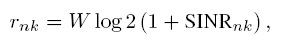
where W denotes the bandwidth of PRB (180KHz) and  is The received SINR for user
  from BS
  on one PRB. The number of consumed resources for each BS according to the practical rate requirement of each user is given by
  =
=  /
/  , where is the practical rate of user k.
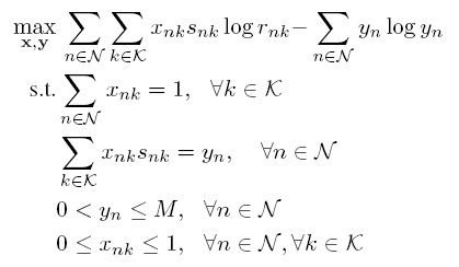
We formulate the following optimization problem that association indicators can be found by maximizing the network-wide aggregate weighted utility function.
where X = {  ,
, 
 } ;
} ; 
 is the total load of BS
  ;
; 
 if the constraint of total resource for BS . Then, we consider the fact of =
  .
.
3. Association Algorithm
As we relaxed the association indicator variables, the combinatorial problem is converted into a convex optimization problem. For the optimal solution of the problem, the corresponding Lagrange function can be expressed as:
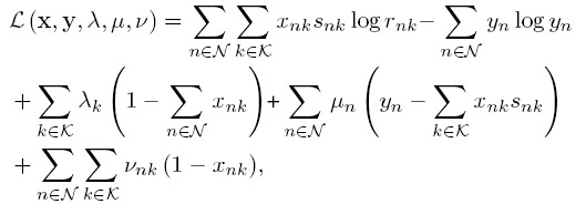
where  = {
= {  , },
, },  = {
= {  , } and
  = {
= {  , , } are the Lagrange multiplier vectors. The objective function of the dual problem can be defined as:

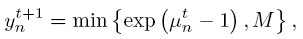
Since the primal problem is a convex optimization problem, a strong duality exists. The association indicator and load of BS can be obtained by applying Karush-Kuhn-Tucker (KKT) conditions, and we have:

where  is sufficiently small fixed step size for updating ; the notion
 ![$[z]^{+}$](ECE_602_Amr_and_Manaf_eq68920.png) represents a projection on the positive orthant, which is used to account for the case that z
represents a projection on the positive orthant, which is used to account for the case that z  0. Then, the optimum values of the above Lagrange multipliers that provide the optimum load distribution can be calculated by solving the dual problem with gradient descent method, and get:
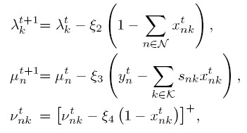
where  ,
,  and
and  are sufficiently small fixed step size for updating , and , respectively. There is a convergence guarantee for the optimum solution since the gradient of the problem satisfies the Lipchitz continuity condition.
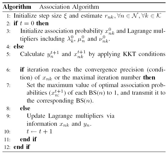
As shown in the algorithm, after getting the optimum association probability, each user selects some BS with maximum association probability .
4. Repreducing Simulation Results
In the following simulation section, We try to reproduce the main results of the assigned paper.
- 4.1 Initialization of Simulation Parameters
We consider a two-tier HCN with transmit power {p1, p2} = {46, 30} dBm. For the propagation environment, we adopt path loss model PL(d) = 128.1 + 37.6 log 10 (d) and PL(d) = 140.7 + 36.7 log 10 (d) for Micro-BS and Pico-BS respectively, where d is the distance between the user and BS in kilometers. In our simulation, the noise power spectral density is set to be 174dBm/Hz and system bandwidth is 20MHz.
clc;
clear;

for loop_i = 1:6
%Total number of User Equipments
no_of_UE = 20 + ((loop_i-1) * 20);
array_UE(loop_i) = no_of_UE;

iteration               = 100000;

%Pico-Cell parameter
no_of_FBs               = 5  ;
Tx_Fpower_in_dbm        = 30 ;


%Macro-Cell parameter
no_of_MBs              = 1 ;
Tx_Mpower_in_dbm       = 46 ;


%algorithm parameter design
BW                         = 180 * 10^3 ;     %one resource block
System_BW                  = 20  * 10^6 ;     %Total B.W of System
Max_resources              = System_BW / BW ; %Total amont of resources reserved for each BS
constant1                  = 0.000001 ;
constant2                  = 0.000001 ;
constant3                  = 0.000001 ;
constant4                  = 0.000001 ;


%additional parameter
uplink_max_power_dbm        =  23 ;
uplink_target_SINR          =  10 ;
noise_power_in_dbm          =  174 ;
no_of_bs                    =  no_of_MBs +  no_of_FBs ;  %Total number of Base-Stations


%dual variable initialization
lamda                 = 0.5 .* ones(no_of_UE , 1);
alpha                 = 0.5 .* ones(no_of_UE , no_of_bs);
beta                  = 0.5 .* ones(no_of_bs , 1);


%primal variable initialization
SINR                           =  zeros(no_of_bs , no_of_UE);


%power in watt and some initial calculation
Tx_Mpower                      =  10 ^ ((Tx_Mpower_in_dbm - 30) / 10) ;              %Macro-cell Transmit Power
Tx_Fpower                      =  10 ^ ((Tx_Fpower_in_dbm - 30) / 10) ;              %Pico-cell Transmit Power
uplink_max_power               =  10 ^ ((uplink_max_power_dbm - 30) / 10) ;          %UE Max. Transmit power
uplink_target_SINR_in_watt     =  10 ^ ((uplink_target_SINR) / 10) ;                 %Target SINR
noise_power_in_watt            = (10 ^ (-1*(noise_power_in_dbm + 30) / 10)) * BW ;   %Noise power
start_of_femto                 = no_of_MBs + 1 ;
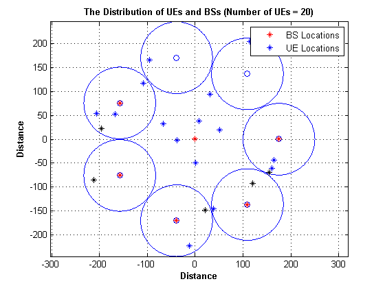
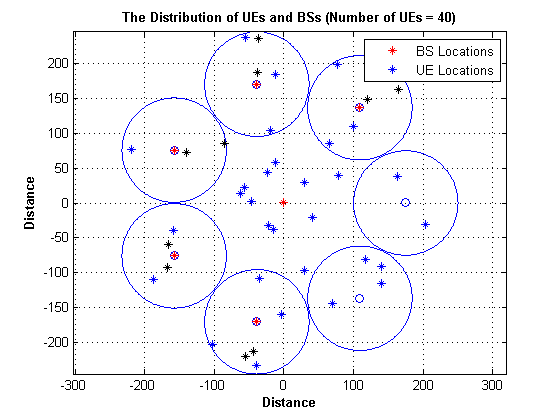
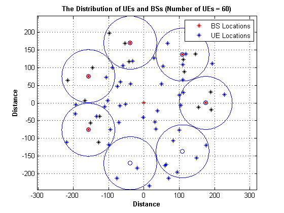
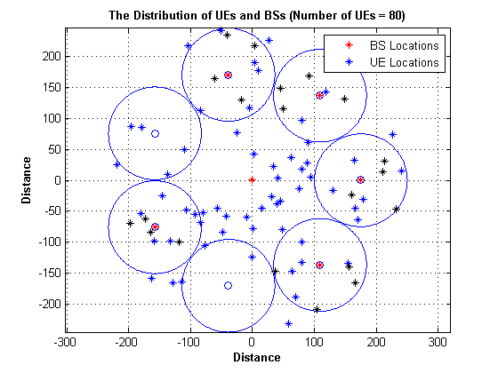
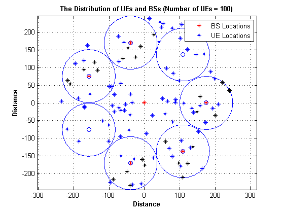
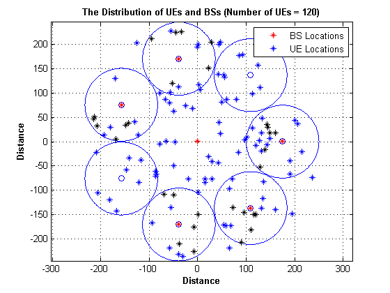
- 4.2 Distriution of User-Equipments and Base-Stations
We first produced a code to generate the distribution of UEs and BSs, and make sure that at least a specified percent of the total number of UEs are located in the Pico-Cells' coverage range. In this HCN, the location of Macro-BS is fixed to form a conventional cellular network (centered at the origin), whereas Pico-BSs and users are scattered into the macrocell in a random way. We set the inter-site distance to be 1000m for the Macro-BSs, and deploy 5 Pico-BSs for each macro-cell.
%Pico-Cell parameter
no_of_pico               = no_of_FBs;
radius_of_pico           = 75;
percent_of_UE            = 1/4;


%Macro-Cell parameter
radius_of_macro       = 250 ;
no_of_MBs             = 1 ;


%algorithm parameter design
mini_dist_pico_macro  = 100 ;
mini_dist_MU_MBS      = 35 ;
edge_dist             = 10 ;

%additional parameter
no_of_bs              =  no_of_MBs +  no_of_pico   ;


%primal variable initialization
dist_Bs_UEIOTD             = zeros(no_of_UE , no_of_bs);
diameter_of_pico           = 2 * radius_of_pico ;

%define all possible Pico cell in macrocell coverage area
no_of_cocentric            = floor((radius_of_macro - mini_dist_pico_macro) / diameter_of_pico );
t                          = linspace(0, 2*pi, 400);
ct                         = cos(t);
st                         = sin(t);
 for i = 0 : no_of_cocentric-1
     if i == 0
     radius = mini_dist_pico_macro + i * radius_of_pico + radius_of_pico ;%na2s ytara7 radius mn hena
     else
     radius = mini_dist_pico_macro + i * diameter_of_pico + radius_of_pico   ;
     end
 end
 for i= 0 : no_of_cocentric-1
     length_of_circle(i+1 , 1) = 2 * pi * (mini_dist_pico_macro + i*diameter_of_pico+radius_of_pico);
 end
 for cir = 0 : no_of_cocentric-1

     radius                       = mini_dist_pico_macro + cir * diameter_of_pico+radius_of_pico ;
     unit_angle                   = asin(radius_of_pico / radius);
     length_of_arc                = radius * 2 * unit_angle  ;
     no_of_aval_pico(cir+1 , 1)   = floor(length_of_circle(cir+1 , 1) / length_of_arc );
     actual_length                = no_of_aval_pico(cir+1 , 1) *  length_of_arc ;
     remaining                    = (length_of_circle(cir+1 , 1) - actual_length )  ;
     remaining1                   = remaining / no_of_aval_pico(cir+1 , 1) ;
     length_of_arc1               = radius * 2 * unit_angle +remaining1 ;
     unit_angle_1                 = length_of_arc1 / radius ;

     for k = 1 : no_of_aval_pico(cir+1 , 1)
         if cir == 0
             row = k ;
         else
             row = k + sum(no_of_aval_pico(: , 1)) - no_of_aval_pico(cir+1 , 1);
         end
          x_coord = (radius * cos((1 * (k-1) * unit_angle_1)));
          y_coord = (radius * sin((1 * (k-1) * unit_angle_1)));
          pico_on_circle(row , :) = [x_coord  y_coord] ;
     end
 end

 figure(loop_i);
 plot(pico_on_circle(: , 1) , pico_on_circle(: , 2), 'o')
 axis equal;
 axis auto;
 grid on;
 hold on;

 t = linspace(0, 2*pi, 400);
 for mm = 1 : sum(no_of_aval_pico)

     ct = radius_of_pico * (cos(t))+ pico_on_circle(mm , 1);
     st = radius_of_pico * (sin(t))+ pico_on_circle(mm , 2);
     plot( ct, st)
     hold on

 end


 %select desired number of Pico cell and determine location for each BS
 pico_on_circle1     = pico_on_circle ;
 M_location          = [0 0] ;
 pico_position      = randi(sum(no_of_aval_pico) ,no_of_pico , 1 );

 for rr= 1 : no_of_pico

     while (pico_on_circle1(pico_position(rr , 1),1)==0 && pico_on_circle1(pico_position(rr , 1),2)== 0 )
         pico_position(rr,1)= randi(sum(no_of_aval_pico),1);
     end

     location_of_pico(rr,:)  = pico_on_circle1(pico_position(rr,1) , :) ;
     pico_on_circle1(pico_position(rr , 1),1) = 0 ;
     pico_on_circle1(pico_position(rr , 1),2) = 0 ;

 end

   bs_location         = [M_location ; location_of_pico] ;

   plot(bs_location(:, 1) , bs_location(:, 2), 'r*' )
   hold on;

 no_of_UED_p         = floor((percent_of_UE * no_of_UE)/no_of_pico);
 no_of_UED_m         = no_of_UE - (no_of_UED_p * no_of_pico );

 %determining location of users and iot devices in Macro
 theta               = 2 * pi * rand(no_of_UED_m , 1) ;
 dist                = (radius_of_macro-mini_dist_MU_MBS) * rand(no_of_UED_m , 1);
 UED_location_m      = [((dist+ mini_dist_MU_MBS) .* cos(theta)) , ((dist + mini_dist_MU_MBS) .* sin(theta)) ] ;
 plot(UED_location_m(: , 1) ,UED_location_m(: ,2) , 'b*')
 hold on;

 %determining location of user in Pico
 for o = 2 : no_of_pico + 1

 theta             = 2 * pi * rand(no_of_UED_p , 1) ;
 dist              = (radius_of_pico - edge_dist) * rand(no_of_UED_p , 1);
 UED_location_p    = [((dist+edge_dist) .* cos(theta)) + bs_location(o , 1) ...
                    , ((dist+ edge_dist) .* sin(theta)) + bs_location(o , 2) ] ;
 plot(UED_location_p(: , 1) ,UED_location_p(: ,2) , 'k*')
 hold on;

 if o == 2
    p = 0 ;
 else
       p = (no_of_UED_p * (o-2))  ;
 end
 for kk= 1 : no_of_UED_p

      UED_location_p_all(p+kk , :) = UED_location_p(kk , :);

 end
 end


 UED_location_in_coverage = [UED_location_m ; UED_location_p_all] ;
 UEIOTD_location = UED_location_in_coverage;


%calculation of location of each user with each base station
for j= 1 : no_of_bs
for i= 1 : no_of_UE

    dist_Bs_UEIOTD(i,j)     = sqrt(sum((bs_location(j , :) - UEIOTD_location( i, :)).^2));

end
end

 title(['The Distribution of UEs and BSs (Number of UEs = ', num2str(no_of_UE), ')'], 'fontweight','bold');
 xlabel('Distance', 'fontweight','bold');
 ylabel('Distance', 'fontweight','bold');
 L = zeros(2,1);
 L(1)= plot(NaN, NaN, 'r*');
 L(2)= plot(NaN, NaN, 'b*');
 legend(L, 'BS Locations', 'UE Locations')
 hold off ;

% The Final UEs and BSs Distriution in Km
dist_Bs_UEIOTD = dist_Bs_UEIOTD .* 10^-3 ;
- 4.3 Solving the Optimization Problem
After solving the optimization prolem and getting the optimum association probability, each user selects some BS with maximum association probability .
%calculating the path loss between each user and each basestation
pathloss_Macro                            =  (128.1  + 8 + (37.6 .* log10(dist_Bs_UEIOTD))) ;
pathloss_Femto                            =  (140.7  + 8 + (36.7 .* log10(dist_Bs_UEIOTD))) ;
pathloss_matrix                           = pathloss_Macro ;
pathloss_matrix(: , start_of_femto : end) = pathloss_Femto(: , start_of_femto : end) ;
path_loss_inwatt                          = 10 .^((-1 .* pathloss_matrix) ./ 10 );
path_loss                                 = path_loss_inwatt';


%calculating signal to interference noise ratio and acheviable data rate
for bs = 1 : no_of_bs
    for device = 1 : no_of_UE
        interference = 0 ;
        if bs == 1
            downlink_power = Tx_Mpower ;
        else
            downlink_power = Tx_Fpower;
        end
        numerator_SINR = downlink_power * path_loss(bs , device) ;
        %calculating denominator of SINR
        for bss = 1 : no_of_bs
            if bss ~= bs
                if bss == 1
            downlink_power1 = Tx_Mpower ;
            interference    = interference + downlink_power1*path_loss(bss,device);
               else
            downlink_power1 = Tx_Fpower;
            interference    = interference + downlink_power1*path_loss(bss,device);
                end
            end
        end
           denominator_SINR = interference + noise_power_in_watt ;
           SINR(bs , device ) = numerator_SINR / denominator_SINR ;

    end
end

% The achievable rate [in Kbps] for user k from BS n
achievable_rate_RB          =  BW .* log2(1 + SINR ) ;


%calcualting needed uplink power for all devices to reach target SINR
uplink_power_limit          = (uplink_target_SINR_in_watt *  noise_power_in_watt)...
                              ./ (10 .^((-1 .* pathloss_matrix) ./ 10));
uplink_power_limit          = min(uplink_max_power,uplink_power_limit);


% An Initial Association Matrix
Initial_matrix = zeros(no_of_UE, no_of_bs);
for q = 1 : no_of_UE
    initial_value = 5000 ;
    for z = 1 : no_of_bs
        if ( dist_Bs_UEIOTD(q , z) < initial_value)
            initial_value = dist_Bs_UEIOTD(q , z);
            initial = z;
        end
    end
    Initial_matrix(q, initial) = 1;
end
Association_matrix          =  Initial_matrix ;


% The practical rate of user k
Dk_matrix = zeros(no_of_UE, no_of_bs);
for q = 1 : no_of_UE

    user_K_initial = randi([0,floor(2*exp(3))]);

    for bs = 1 : no_of_bs
    Initial_Dk_matrix(q, bs) = user_K_initial ;
    end

end
Dk_matrix          =  Initial_Dk_matrix * 10^3 ;


% The load of user k on BS n
Snk_Matrix = transpose(Dk_matrix) ./ achievable_rate_RB ;


%%%%%%%%%%%%%%%%%
% The Algorithm %
%%%%%%%%%%%%%%%%%

for it = 1 : iteration

    Previous_Association_matrix = Association_matrix ;

% The new Association Matrix
for k = 1 : no_of_UE
    for n = 1 : no_of_bs

        Association_matrix(k , n) = Association_matrix(k , n)...
            +(constant1 * ( ( Snk_Matrix(n , k) * log( achievable_rate_RB(n , k)))...
            - lamda(k , 1) -  ( beta (n , 1) * Snk_Matrix(n , k)) - alpha(k,n))) ;

        Association_matrix(k , n) = max(Association_matrix(k , n) , 0);

    end
end

% The new Effective load
for r = 1 : no_of_bs
  effective_load(1 , r) = min(exp( beta(r , 1) - 1) , Max_resources);
end

% Check the convergence
if (max(Previous_Association_matrix - Association_matrix) < 0.00000001)
    break;
end

%update dual variable
for k = 1 : no_of_UE

   lamda(k , 1) = lamda(k , 1)- (constant2 * (1 - sum(Association_matrix(k , :)))) ;

end

Ynk_Matrix = transpose(Snk_Matrix) .* Association_matrix ;
new_effective_load              =  sum(Ynk_Matrix,1) ;
for n = 1 : no_of_bs

   beta(n , 1) = beta(n,1) -    (constant3 * (effective_load(1,n) - new_effective_load(1,n)))  ;

end

for k = 1 : no_of_UE
    for n = 1 : no_of_bs

        alpha(k,n)   = alpha(k,n) - (constant4 * (1 - Association_matrix(k , n)));
        alpha(k , n) = max(alpha(k , n),0);

    end
end

end


%%%%%%%%%%%%%%%%%%%%%%%%%%%%%%%%%%%%%%%%%%%%%%%%%%%%%%%%%%%%%%%%%%%%%%%%%%%%
Ynk_Matrix                     = zeros(no_of_UE , no_of_bs);
Association_matrix_rounding    = zeros(no_of_UE , no_of_bs);

Ynk_Matrix = transpose(Snk_Matrix) .* Association_matrix;

loc           = zeros(no_of_UE,1);
for u = 1 : no_of_UE

    [maxvalue , loc(u,1)]= max(Association_matrix(u , :));
    if (maxvalue ~= 0)
    Association_matrix_rounding(u ,loc(u) )= 1 ;
    end
end


Association_indicator = Association_matrix_rounding ;


Ynk_Matrix                = transpose(Snk_Matrix) .* Association_indicator ;
effective_load_Last       =  sum(Ynk_Matrix,1);
load_Balancing_Index = ( sum(effective_load_Last) )^2 / (no_of_bs * sum(effective_load_Last.^2)) ;


%%%%%%%%%%%%%%%%%%%%%%%%%%%%%%%%%%%%%%%%%%%%%%%%%%%%%%%%%%%%%%%%%%%%%%%%%%%%%%
arr_index_1(loop_i) = load_Balancing_Index ;
end
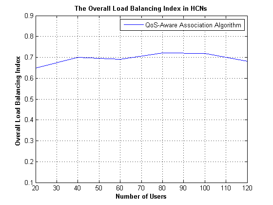
- 4.4 The Final Simulation Results
In order to explore the effect of QoS requirements on the association performance, we consider Qos-Aware association strategy.
figure(loop_i + 1);
plot(array_UE, arr_index_1)
axis auto;
grid on;
title('The Overall Load Balancing Index in HCNs', 'fontweight','bold');
xlabel('Number of Users', 'fontweight','bold');
ylim([0.1 , 0.9]);
ylabel('Overall Load Balancing Index', 'fontweight','bold');
legend('QoS-Aware Association Algorithm')
hold off ;
5. Concluding Remarks
In this project, We have reproduced the main results of the assigned paper. The results obtained are consistent with the results presented in the paper. According to the reproduced results, we can make the same key observations as in paper [1]. Nevertheless, here are several aspects to clarify:
(a). We first wrote a code to generate the User-Equipments (UEs) and Base-Stations (BSs) Distribution (not included in the paper) to insure that at least a specific percent of UEs are located inside the small cells.
(b). As the authors do not specify the simulation nodes distribution settings in this paper, the parameters used in this project are very likely to be different from the original paper. Thus, the results or settings of this project are slightly different from the original paper.
(c). In the paper, authors compare their algorithm "QoS-Aware Association" with two other algorithms in two different papers; I reproduced in this project the "QoS-Aware Association" algorithm only. However, the code of other two algorithms can be easily implemented by adapting existing implementations.
6. References
[1] T. Zhou, Y. Huang, L. Yang, "QoS-aware user association for load balancing in heterogeneous cellular networks", Proc. IEEE VTC Fall, pp. 1-5, Sep. 2014.